1 Introduction to optimal control
In the past lectures, although we have designed controllers based on some criteria, but we have never considered optimality of the controller with respect to some index. In this context, Linear
Quadratic Regular is a very popular design technique.
The optimal control theory relies on design techniques that maximize or minimize a given performance index which is a measure of the effectiveness of the controller.
Euler-Lagrange equation is a very popular equation in the context of minimization or maximization of a functional.
A functional is a mapping or transformation that depends on one or more functions and the values of the functionals are numbers. Examples of functionals are performance indices which will be introduced later.
In the following section we would discuss the Euler-Lagrange equation for discrete time systems.
1.1 Discrete Euler-Lagrange Equation
A large class of optimal digital controller design aims to minimize or maximize a performance index of the following form.
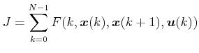
where ![]() is a differentiable scalar function and
is a differentiable scalar function and ![]() ,
,
![]() .
.
The minimization or maximization of J is subject to the following constraint.
![]()
The above can be the state equation of the system, as well as other equality or inequality constraints.
Design techniques for optimal control theory mostly rely on the calculus of variation, according to which, the problem of minimizing one function while it is subject to equality constraints is solved by adjoining the constraint to the function to be minimized.
Let ![]() be defined as the Lagrange multiplier. Adjoining J with the constraint equation,
be defined as the Lagrange multiplier. Adjoining J with the constraint equation,
![$\displaystyle {J}_a = \sum\limits_{k = {0}}^{{N-1}} F(k, \boldsymbol{x}(k), \bo... ...da}(k+1), [\boldsymbol{x}(k + 1) - f(k, \boldsymbol{x}(k), \boldsymbol{u}(k))]>$](images/img8.png)
where ![]() denotes the inner product.
denotes the inner product.