Calculus of variation says that the minimization of J with constraint is equivalent to the minimization of Ja without any constraint.
Let ![]() and
and ![]() represent the vectors corresponding to optimal trajectories. Thus one can write
represent the vectors corresponding to optimal trajectories. Thus one can write
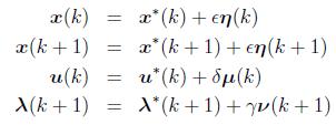
where ![]() are arbitrary vectors and
are arbitrary vectors and ![]() are small constants.
are small constants.
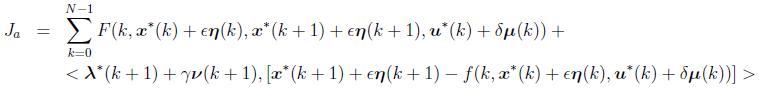
Substituting the above four equations in the expression of Ja,
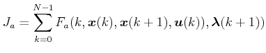
To simplify the notation, let us denote Ja as
![]()
Expanding Fa using Taylor series around ![]() and
and ![]() , we get
, we get
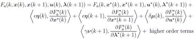
where
![]()
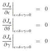
The necessary condition for Ja to be minimum is