Module 1: General Introduction – Continuum Damage Mechanics (CDM)
LECTURES 1 – 6
- Continuum-Damage-Mechanics,
- Physical nature of damage,
- mechanical representation of damage,
- Measurement of damage,
- Engineering Applications,
- General scope of Continuum Damage Mechanics
Key-words: Contiuum-Damage, Manifestation of damage, measurement of damage, Applications of CDM
Introduction
The success of an engineering design often depends on an appropriate selection of a specific material with respect to its mechanical, magnetic, heat conduction, optical and other physical properties. The desired level of its mechanical strength and economy are more often than not the primary considerations in the choice of one among available structural materials for a particular application.
Until very recently all Codes and Standards were based, almost without exception, on the elastic behavior of the material. The only material properties of any interest were the elastic and shear modulus and the proportional yield limit of the material. The wide safety margins inherent to this design philosophy (when applied to ductile materials) effectively discouraged inquiries into the true behavior of the solids, relegating the research into the inelastic material theories to the more rarefied atmosphere of the academic world. However, the ever increasing demands placed by modem industry on the materials, which more and more frequently had to cope with hostile thermal and chemical environments, coupled with the emphasis on economy (reflecting the diminishing resources) presented a strong incentive to re-examine the general design philosophy of the governing Codes and Standards.
The often inflated safety margins were the first and obvious target. By their very nature, the safety margins reflect the three basic uncertainties: those associated with the magnitude and character of the often non-deterministic loads, those associated with the often not well understood or not well controlled material properties and defects and, finally, those associated with the inevitable assumptions and simplification on which the analytical models are based. The advent of powerful computing devices in conjunction with the development of the numerical methods packaged into ready-to-use computer codes are well along their way to solving the computational aspects of the stress analyses. The inquiry into the actual behavior of the material is less of a success story. Despite some great strides in enriching our arsenal of methods coping with a variety of practically important problems, a continuum mechanics model for fatigue, strain-rate effect, size effect, etc., remains an elusive goal.
The initial effort in sorting out the mysteries of the nonlinear behavior of solids was developed almost exclusively within the framework of the theory of plasticity. Being in many ways the only reputable theory of the nonlinear behavior of the materials which at that moment in time had a rigorous continuum mechanics foundation, the theory of plasticity was certainly the most logical choice for the task of developing a tool to deal with an often bewildering array of phenomena of great theoretical and, more importantly, practical interest. Popularity being what it is, it did not take long before the theory of plasticity was stretched beyond the limits of its applicability. Cracking at its seams, the theory of plasticity was endlessly modified in order to satisfy the hunger of many authors trying to use the venerable old theory to describe the mechanical response of materials such as rocks, concrete, ceramics, granular materials, clays, sands and many other under a variety of circumstances. While the ductility of those materials is a matter of imagination, the vestiges of the time gone by die slowly. According to some, the theory of plasticity, in one of its many incarnations, is still a panacea to be used whenever the stress-strain curve demonstrates the slightest tendency to deviate from a straight line.
Bolstered by the recent advances in electron scanning microscopy, acoustic emission technique and a host of other newly developing methods of non-destructive testing, a strong conviction is emerging that the material response of solids to a large extent depends not only on the basic structure of the matrix but also on the type and distribution of defect in the matrix. The objective of this study is to emphasize this point and to discuss a relatively new branch of continuum mechanics known as the continuum damage theory. While the name continuum damage mechanics (CDM) was apparently coined by Janson and Hult (1977), the theory itself can be traced back, according to consensus, to its progenitor L. Kachanov (1958). A host of already resolved problems (some of which will be discussed at length within this study) and a long list of names associated with the continuum damage theory are testimony to its obvious intuitive appeal and physical clarity. A number of recently held workshops, ASME, ASCE, IUTAM and Euromech symposia, the 1986 CISM course, etc., lend further credence to the opinion of many that continuum damage mechanics is not a passing fad. One wonders whether a journal on damage mechanics can be far behind.
Continuum damage mechanics: What, when and why?
Damage mechanics is one of the most important and interesting branches of solid mechanics: although it is still developing, it has already been applied to many engineering problems. The pioneer of the damage parameter proposal was Murzewski, who put forward a probabilistic interpretation of the decohesion parameter. Following in his footsteps, Kachanov, then Rabotnov formulated the famous equation of damage growth under creep conditions for the uniaxial state of stress. The theory was formulated in the 1950’s and one of the first papers in the Western scientific literature was published by Odqvist and Hult in the early sixties. Since that time, a number of theoretical and experimental investigations have been performed; see e.g. Chrzanowski, Chaboche , Krajcinovic and Lemaitre .
Continuum Damage Mechanics was initiated by Kachanov in 1958 to model creep damage in metals. The theory considered the description of state variables in the framework of thermodynamics of irreversible process. This immediately caught attention of contemporary researchers as a very good tool for description of various types of damage in materials. Number of models are now available for various types of materials including metals, laminated fibre reinforced composites, concrete, rocks, etc.
Every time the development of a new branch of continuum mechanics is advocated, the question of why such an endeavor is undertaken and what the hypothetical benefits of such an effort are more to be addressed. Every new theory is supposed to provide answers to unresolvable problems by existing theories, and to be able to predict the salient trends of the material behavior of a reasonably wide class of solids over a sufficiently large set of circumstances. While the engineering practice is usually satisfied with predictions in a phenomenological sense, it is probably just as important to require that a particular theory in some average or smoothed sense models the kinetics of the physical phenomena on which the phenomenological (macroscopic) response is based.
Although the details of the material behavior will be discussed at some length at a more appropriate place (Section 3), a short precise seems to be in order as a part of these introductory remarks. In principle, the elastic parameters of a solid can be determined from the interatomic forces bonding at the atoms together (ionic, homopolar (A covalent bond whose total dipole moment is zero.) and metallic bonds, in particular (see Billington and Tate, 1981)). In other words, the elastic parameter of a polycrystalline material fully depends on the type of constituent crystal which is in turn a stable mechanical system of atoms held together by interatomic forces. On the other hand, the nonlinear response of the solid and ultimately its mechanical strength are dependent on the type, distribution, size and orientation of the defects in its structure. For example, the theoretical shear strength of a perfect crystal is two to three orders of magnitude larger than the shear strength measured in experiments on polycrystalline materials containing the same crystals. Thus the yield stress is a structure-sensitive property of the solid (along with fracture and creep strength, electrical conductivity and semiconductor properties (see Dieter, 1976). As already stated, the elastic constants, along with the density, melting point, specific heat and coefficient of thermal expansion, are the structure (defect)-insensitive material properties.
Even though the elastic properties of the material, depending on the properties of the material in its virgin state, have but a tenuous relation to strength at rupture, the existing AISC Code stubbornly persists in legalizing the myth on the causal relation between the modulus of elasticity and rupture strength. While a misconception like this, canonized into a code, has a tendency to linger on, it is hoped that a study of this type will help in pointing out the need for the re-examination of some of the traditional empirical models of material behavior.
Material (lattice) defects can be roughly classified with respect to their geometry into point defects (vacancies, interstitial and impurity atoms), line defects (dislocations), plane defects (slip planes and cracks) and volume defects (pores and cavities). Inelastic deformation is also the result of twinning, stacking faults, phase changes, diffusional flow, etc. From a purely practical viewpoint, it is convenient to classify most of these defects into two large groups responsible for what is commonly known and defined as the brittle and/or ductile behavior. Naturally, no material is either totally ductile or perfectly brittle. The degree of ductility in all probability depends on the extent to which a particular mode dominates the process of deformation (or energy dissipation). The same material can be either brittle or ductile depending on the circumstances. A concrete or rock specimen in unconfined uniaxial compression will behave in a brittle manner and will ultimately fail in the splitting mode. The same specimen when confined will behave in a ductile manner and will fail only after developing visible shear bands. Additionally, temperature enhance ductility (lowering the glide resistance), while an increasing rate of loading promotes increasing brittleness.
At some danger of oversimplification, the basic features of ductile and brittle behavior may be arranged into a table such as the one shown below.
The fundamentally different way in which the two classes of microstructural defects influence the macrostructural response of a solid casts serious doubt on the applicability of the theory of plasticity (reflecting the influence of slips over active crystalline slip planes on the deformation) to solids such as rock or concrete responding in a predominantly brittle mode (characterized by the fact that most of the energy is dissipated in the nucleation and propagation of microcracks). Regardless of the skill in modifying the plasticity theory, the fact remains that the history is recorded by some combination of residual strains and that the onset of inelastic deformation is related to exceeding some glide resistance according to the plasticity theory. Neither of these aspects have anything in common with the response of solids in the brittle mode.
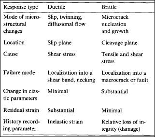
Table 1.1: Ductile and brittle response of solids
The relation between continuum damage mechanics and fracture mechanics is in many ways contingent on the selected model and scale rather than on the fundamental difference between the involved phenomena. For example, the question of whether conventional fracture mechanics can be applied to concrete is a more insidious one and, as such, is still a matter of considerable debate (see, for example, Mindess, 1983). Rephrased occasionally as a question of whether the stress intensity factor and the J integral are the material parameters, the problem is typically approached in a somewhat biased manner considering notched specimens. Anticipating the scale effect and the difference between macro- and microcracks, the problem appears to be how much the behavior of concrete specimens with notch and without notch are common. Or to put it more succinctly, whether the ratio of the energy dissipated by the nucleation and growth of microcracks (evolution of the process zone in the parlance of the concrete literature) and the energy needed for the growth of the macrocrack is in the case of the specimens with notch and without notch at least similar, if not identical. The intuitive feeling, fortified by the experimental results of Pak and Trapeznikov (1982), who determined the minimum crack size below which the Griffith-Irwin fracture mechanics theory is not valid, is that this ratio depends on whether the specimen is notched or not. Thus at least a partial resolution of the controversy discussed in Mindess (1983) may rest on an almost trivial conclusion that fracture mechanics will apply to concrete specimens with notch but not to specimens without notched one.
The situation is by no means unique to concrete. The Evans and Faber (1984) results indicate the same trend in alumina ceramics where the toughness was found to be strongly dependent on the extent of the 'process zone', i.e., the grain size. The results of Hoagland et al. (1973) for rock showed that a much larger part of the energy is dissipated in microcracking than in the propagation of a few well developed macrocracks. The same conclusion was reached by Meyers (1985) who found that the total surface area of internal (micro) cracks is at least an order of magnitude higher than the surface area of fragments. Since the crack surfaces translate into dissipated energy, the conclusion is that a theory solely considering macrocracks will miss most of the action. A similar situation was found to exist in polymers as well, and the differences in the experimental measurements of the critical stress intensity factors and J integrals could not be ascribed to the normal dispersion of test data. According to Table 9 in Kausch (1978) using different experimental techniques, the measurements of the critical stress intensity factor may differ by a factor of 50. Even in the case of metals, a cursory look at the micrographs of uniaxially stretched copper specimens published by Leckie and Hayhurst (1974) would suffice as a strong indication that the extent of microcracking in the 'process zone' surrounding the macrocrack tip presents a strong energy sink which cannot be neglected without a significant, and probably unacceptable, loss of accuracy. The progressive deterioration of the 2024 steel alloy in tensile experiments (Lemaitre and Chaboche, 1978) is clearly reflected in the decrease of 'elastic' (unloading) moduli of up to 22%.
The evidence relating to the influence of microcracks on the mechanical response of solids over a wide spectrum of circumstances is too obvious to be neglected. Even though phenomena such as the lateral splitting of concrete and rock specimens in uniaxial compression or the tertiary creep of metals can be modeled by some fitting procedure, the hard fact remains that these and many other effects reflect microcrack nucleation and growth in solids.
The objective of this study is to suggest that damage mechanics is a rational framework for dealing with problems characterized by the dominant role of microcracking in energy dissipation. For the purpose of discussion, a particular model will be regarded as a damage model only if it features a special internal variable which in some manner qualifies (if not quantifies) the microcrack density and distribution (or the state of damage) locally, and a kinetic equation defining the evolution of the 'damage' with the applied load or time. In view of the already discussed fact that the inelastic (residual) strain is a poor choice to record the history, the decision to exclude some models from further consideration is not purely formal in nature. On the other hand, the so-called passive
(or non-process) models focusing on the determination of the stiffness of a specimen weakened by a given pattern of defects (Delameter and Herrmann, 1974; Salganik, 1975; Budiansky and O'Connell, 1976; Horii and Nemat-Nasser, 1983, etc.) and lacking the kinetic equation will be discussed only in the context of the general theory.
In summary, the damage theory should be applied either alone when the response is primarily brittle, or in conjunction with other theories such as plasticity if the response in neither perfectly brittle nor ductile, or fracture mechanics if a large well-developed crack interacts with a large number of microcracks surrounding its tip. A particular damage theory may be either phenomenological or micromechanical in nature. In either case, though, it is felt that the model must at the very least be motivated by the actual geometry of the defects and the kinetics of the changes on the grain or crystal scale. Having in mind the existence of some well established theories of porous solids, it seems reasonable to place strong emphasis on the crack-like (high aspect ratio) defects.
Fracture and Damage
Failure description in materials has been recognized to be of vital importance since long. Tracking failure up to rupture of component is of extreme significance while trying to estimate the health and remaining life of any structure. Fracture Mechanics classifies crack propagation in three fundamental modes, viz. Mode I, Mode II and Mode III. Failure in most cases is mixed mode, subsequently leading to a predominant crack expansion in Mode I. Fracture Mechanics approach has been favoured since its advent owing to the sound mathematical treatment given to the plasticity around crack tips and the energy dissipated in creation of new crack surfaces.
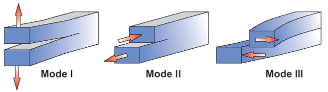
Figure 1.1: Opening, Sliding and Tearing Fracture Modes
Mode 1: Opening mode (the tensile stress normal to the plane of the crack)
Mode 2: Sliding mode (the shear stress acting parallel to the plane of the crack and perpendicular to the crack front)
Mode 3: Tearing mode (a shear stress acting parallel to the plane of the crack and parallel to the crack front)
The stress intensity factor at a crack tip may be determined by the equation:
………………..(1) |
where; KI = Stress Intensity Factor in Mode I
σ = Applied far field stress
a = Length of existing crack in the continuum
A corresponding material property has to be determined known as Critical Stress Intensity Factor, known as Critical Stress Intensity Factor in mode I KIC. If the value of Theoretical Stress concentration factor Kt at any given value of stress exceeds the critical value KC, then the crack is deemed to propagate, whereas if Kt<KC, the crack will not propagate.
As evident from equation (1), the theory of Fracture Mechanics suffers from a serious drawback in the essential requirement of a non-zero value of crack length. This renders Fracture Mechanics diffi;cult to implement when there is no crack existing in the structure such as a virgin material or when the cracks that exist are of length that can’t be easily detectable by non-destructive testing methods. Accurate determination of cracks having very small length may not be feasible and the error creeping in due to the square root of the crack length may increase the error in determination of the stress intensity factor.
Damage mechanics does not depend on the pre-existence of voids or failure zones. Hence, damage mechanics is rapidly becoming the theory of choice for description of failure in important structural components such as aircraft fuselage, propeller blades, etc.
Phenomenological Aspects//Damage at a Point (Physics and Damage Variables)
Damage, in its mechanical sense in solid materials is the creation and growth of microvoids or microcracks which are discontinuities in a medium considered as continuous at a larger scale. In engineering, the mechanics of continuous media introduces a Representative Volume Element (RVE) on which all properties are represented by homogenized variables. To give an order of magnitude, its size can vary from about 0.1 mm in metals and ceramics to about 100 mm in concrete. The damage discontinuities are “small” with respect to the size of the RVE but of course large compared to the atomic spacing (Figure. 1.2).
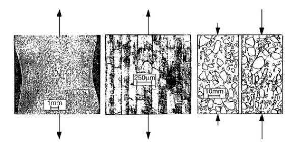
Figure 1.2: Examples of damage in a metal (left, micro-cavities in copper from L. Engel and H. Klingele), in a composite (middle, microcracks in carbon-fiber/epoxy resin laminate from O. Allix), and in a concrete (right, crack pattern in a ASTM I cement, 4.8 and 9.5 mm aggregates, petrography from S.P. Shah)
In an anisotropic material, damage can be defined as a tensorial entity, requiring the definition of plane on which we are considering damage and the direction vector for considering the developed microfailure. However, for isotropic materials, this simplifies to a vectorial form in which, only the section defining vector is mandatory. If the section is clearly defined by the type of structure and nature of loading, the damage may be defined in scalar form. For example, in a rod under tension, the direction vector for the section is clearly perpendicular to the principal axis of the rod.
Definition of Scalar Damage Variable (D)
At any given material point as shown in Figure 1.3 in a continuum, the value of damage ![]() attached to point M in the direction
attached to point M in the direction ![]() and at abscissa x is:
and at abscissa x is:
|
………………..(2) |
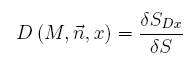
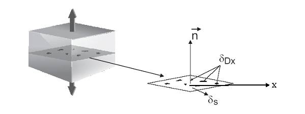
Figure 1.3: Definition of Damage
To define a continuous variable over RVE, for its deterioration to failure, one must examine all planes varying with x and consider the most damaged one. In this sense, the requirement of coordinate x vanishes and damage can then be defined as:
|
………………..(3) |
Equation (3) indicates that a scalar variable D, which depends on the position of material point, the cross section plane and the direction vector, is bounded by 0 and 1:
………………..(4) |
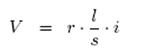
D = 0 indicates a virgin material RVE having no flaws, voids or cracks. On the other hand, D = 1 indicates a completely ruptured RVE. In reality, a material RVE seldom reaches value of D = 1. This is due to the fact that due to instability, the material RVE reaches a stage of uncontrolled damage propagation at a damage value much less than 1. This value is known as Critical Damage variable DC and is typically of the order of 0.3 − 0.4. In fracture mechanics sense, this would correspond to Critical Stress Intensity Factor KIC. For a one-dimensional case, where the area of section can be measured, equation (3) takes the form:
|
………………..(5) |

Equation (5) is extremely useful. Most engineering problems comprise of either isotropic materials. Laminated composites segregate various failure modes and apply the 1-D equation to characterise each mode.
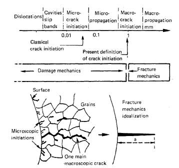
Figure 1.4: (a) Schematics of fatigue crack growth; (b) illustration of microscopic crack initiation
Physical Manifestations of Damage
At the microscale level, damage is governed by only one general mechanism of debonding. However, at the macro scale, it can manifest itself in various ways depending on the type of the structure, nature of loading, temperature, humidity, and other ambient conditions.
Brittle Damage
The damage is termed as brittle when the crack is initiated at the mesoscale without significant amount of plastic strain or absorption of energy. This type of damage is usually observed in brittle materials such as glass. This means that the energy supplied to the material is larger than that required for producing plastic slips, but is enough to initiate cleavage at grain boundaries (or less commonly across the grain boundaries).
The dominant mechanism of brittle damage is the nucleation and growth of microcracks. These cracks usually have a preferred orientation given by the principal axes of the stress tensor. Under tensile loading cracks are observed to grow preferentially normal to the maximum tensile stress (Fig. 9.3). Their characteristic length in the initial state, however, is typically determined by the microstructure of the material (e.g., grain size). In the course of loading and beyond some critical load the cracks start to grow and multiply which leads to a decreasing stiffness (e.g., Young’s modulus) in the direction of loading. Although the undamaged matrix material behaves linear elastic the macroscopic behavior of the damaged material is nonlinear because of the increasing damage (Figure. 1.5). The deformation process proceeds in this way until the material becomes macroscopically unstable and a localization of damage takes place. Damage then is no longer uniformly distributed throughout the material; instead a single crack which dominates over the others continues to grow alone.
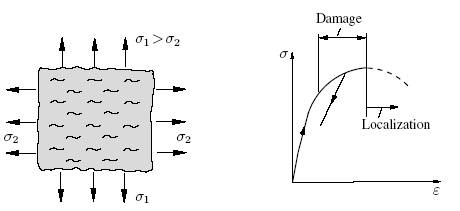
Figure 1.5: Brittle damage under tensile loading
In case of compressive loading, cracks are often observed to grow into the direction of maximum compressive stress (Fig. 9.4a). They may originate from various mechanisms which give rise to local tensile stress fields. A typical example is a spherical cavity or inhomogeneity at the poles of which a local tensile stress is induced under global compressive load. Another mechanism involves shear cracks under mode-II loading which kink and afterwards grow under local mode-I conditions into the direction of overall compression (Figure. 9.6(b)). The macroscopic material behavior again is nonlinear due to the increasing damage and in the course of deformation displays a material instability which leads to the localization of damage. This localization often takes place in form of shear bands which originate from the growth and coalescence of shear cracks and which are inclined at a certain angle to the overall compressive load.

Figure 9.6: Brittle damage under compressive loading
In the following we consider a simple example of damage under uniaxial tension (Figure. 9.7). The RVE is modeled as a plane region of area _A which in the initial state contains only a single mode-I crack. Its length is sufficiently small compared to the distance to other cracks so that the interaction of the cracks need not be accounted for. The macroscopic material behavior is described using the complementary energy.
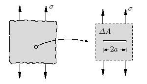
Figure 9.7: 2D model for damage under tensile loading
Ductile Damage
Damage is called ductile when it occurs simultaneously with significant amount of plastic strain at the meso-scale. This type of damage is commonly seen in materials like steel, copper, aluminium or other metals. This mainly results from nucleation of cavities due to decohesions between inclusions and the matrix followed by their growth and coalescence.
Creep Damage
When a material is loaded and the stress is kept constant, the material may deform over time exhibiting damage. Such damage is known as creep damage. This type of damage would be significant mainly when the material is loaded at elevated temperatures, typically above 1/3rd of the melting temperature. At such elevated temperatures, plasticity involves viscosity. The main processes involved in this type of damage are the inter-granular cleavage and decohesions.
Fatigue Damage
When a material is subjected to cyclic loading, the damage may develop due to the incremental nucleation of cracks at grain boundaries. Fatigue damage may be sub-classified in Low Cycle Fatigue and High Cycle Fatigue.
Low Cycle Fatigue
When the cyclic stress is high, the damage develops together with plastic strain. This damage further develops and nucleates into microcracks, which in turn rapidly grow to form meso-level cracks. The degree of localization is high as compared to ductile or creep damage. Due to the high value of stress, the low cycle fatigue is typically characterized by low number of cycles to initiation of damage and subsequent failure. Typically, number of cycles to rupture NR < 10000. For metals, the damage can be either intergranular or transgranular, following slip band arrests.
 |
|
High Cycle Fatigue
When a material is loaded with lower values of stress, the plastic strain at mesoscale level remains small. Plastic strains can be observed in such cases mainly on the surface due to intrusion and extrusion. At micro-scale, it may be high only at certain planes. The number of cycles to rupture is fairly large. As a division, damage is said to be High Cycle Fatigue damage when the number of cycles to rupture NR > 10000.
Mechanical Representation of Damage
In extremely simple terms, damage may be defined as the amount of breakage a material point has undergone due to the applied load system. While this definition is enough to understand the concept of damage, it is vital to understand that the scale at which we are talking makes a huge difference in the perception of damage. For example, in a 20cm steel cube, if there is some damage at a point inside the core, it may not be visible at all on the surface. Now, if we make the cube size smaller and make a cube of say 1cm size, the change in behavior due to that damage may start surfacing. However, it should be kept in mind that the voids and cracks may be of micro-size. This means that the smeared effect of those cracks may be just barely visible at 1cm cube size level. If we go further and study the effect on a 1mm cube size, the effect may become more evident. It should be evident now that a 0.1mm cube size would be ideal to encompass the effect of cracks and also have the cracks show their presence in terms of mechanical properties. This leads to the concept of Representative Volume Element (RVE).
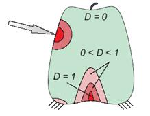
Figure 1.8: Damage Distribution
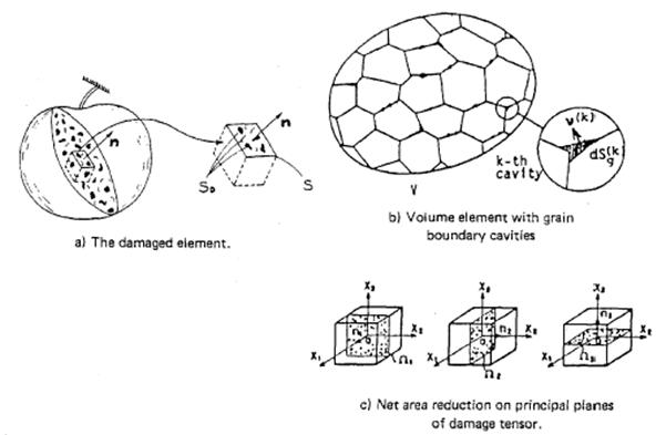
Figure 1.9: Net area reduction: (a) the damaged element; (b) Volume element with ground boundary cavities; (c) net area reduction on planes (where principal stress is acting) of damage tensor
The Representative Volume Element is a cubic element that is small enough to represent the continuum behavior of the material and to avoid smoothing of high gradients, but at the same time, is large enough to encompass and represent an average various micro-processes happening at the micro-structural level. The processes include:
- Elasticity at the level of atoms
- Plasticity (governed by slips) at the level of crystals or molecules
- Damage or debonding from the level of atoms to mesoscale level for crack initiation
From a physical point of view, damage is always related to plastic or irreversible strains and more generally to a strain dissipation either on the mesoscale, the scale of the RVE, or on the microscale, the scale of the discontinuities:
- In the first case (mesolevel), the damage is called ductile damage if it is nucleation and growth of cavities in mesoscale level in plastic strains under static loadings; it is called creep damage when it occurs at elevated temperature and is represented by intergranular decohesions in metals; it is called low cycle fatigue damage when it occurs under repeated high level loadings, inducing plasticity at mesoscale level.
- In the second case (microscale level), it is called brittle failure, or quasi-brittle damage, when the loading is monotonic; it is called high cycle fatigue damage when the loading is a large number of repeated cycles. Ceramics, concrete, and metals under repeated loads at low level below the yield stress are subjected to quasi-brittle damage.
-
For experiments and analytical purposes, it may be useful to consider the following orders of magnitude of Representative Volume Element:
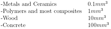
Table 1.2: Indicative (i.e., typical) RVE Sizes
Measurement of Damage
Introduction
The definition of damage describes the amount of voids intersecting a cross section or the total volume of voids in a given unit volume. Such description of damage in mathematical sense may be easier, but physically estimating the damage in a material may not be an easy task. It is important to be able to measure damage at a given point in order to establish the validity of the derived mathematical models trying to describe damage and also to ascertain the physical state of health of the structural component.
The methods for measurement of damage may be broadly classified into two categories, viz. direct measurements and indirect measurements. Various significant methods available for experimental determination of damage at a point are described in subsequent sections.
Direct Measurement
Direct measurement of damage involves cutting of a section from the component and examining it under a high power optical microscope or a scanning electron microscope. Commonly, micrograph pictures are taken and studied.
Damage at a point is defined as ![]() . This equation is actually evaluated at the cross section by cutting a plane across it and measuring the area of voids intersecting the section and the area of cross-section. Care must be taken to take a section of appropriate RVE size as per the material under consideration. To observe a picture of 100 mm2 section of RVE, a maximum magnification of 1000 is deemed suffi;cient for metals and 1 to 10 is considered to be enough for concrete.
. This equation is actually evaluated at the cross section by cutting a plane across it and measuring the area of voids intersecting the section and the area of cross-section. Care must be taken to take a section of appropriate RVE size as per the material under consideration. To observe a picture of 100 mm2 section of RVE, a maximum magnification of 1000 is deemed suffi;cient for metals and 1 to 10 is considered to be enough for concrete.
As obvious, this is a destructive test and hence has its associated drawback of being tedious to implement. Further, there may be non-uniform trapped plastic stresses and strains in the body which may get released when the section is cut. This would not only change the apparent area of voids, but would also change the effective area of cross section. There is also a chance of inducing more damage in the section while cutting the section. Also, cracks which intersect the cross-section will be visible only as lines on the cross section. Such cracks can be considered in an approximate sense only. A method to consider such cracks has been explained by Lemaitre. A detailed treatment to some of the commonly used methods of damage detection has been presented by Lemaitre and Dufailly.
Indirect Measurement
Indirect measurements do not involve most of the problems associated with direct measurements. Of course, the direct measurements are a sure indicator and involve less imprecision errors than indirect measurements. However, indirect measurements have a benefit of being easy to perform and also give damage values with sufficient accuracy. Indirect methods depend mainly on the fact that the properties of materials degrade with increase in damage. This degradation in properties are usually measured and correlated with prevalent damage in the material. However, it should be noted that since indirect measurements involve tracking the degradation of properties, value of initial damage in the material is usually extrapolated from available damage points.
Reduction in Modulus
When a body is strained, the voids or damage increase. This increase in damage reduces the effective area available for load transfer, subsequently reducing the modulus of elasticity. This can be observed in tensile tests involving loading and unloading of the specimen. For example, if a bar specimen is tested in tension under loading and unloading cycles, a typical stress-strain graph would look as shown in Figure 1.5. Close observation will indicate that ![]() .
.
The influence of damage on elasticity modulus through state coupling is given as:
|
………………..(6) |
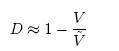
If ![]() is considered to be the effective elasticity modulus of the damaged material, the values of damage may be derived from the measurements of E, provided that the initial Young’s modulus E is known:
is considered to be the effective elasticity modulus of the damaged material, the values of damage may be derived from the measurements of E, provided that the initial Young’s modulus E is known:
|
………………..(7) |

Figure 1.10: Typical Loading-Unloading Tensile Test
Reduction in Micro-Hardness
This method is a non-destructive test and is quite promising. The micro-hardness test consists in indenting a diamond indenter in the material, the hardness H (hardness material parameter) being defined by the mean stress:
|
………………..(8) |
The load F on the indenter is chosen to obtain a projected indented area S of the same order of magnitude as that of the representative volume element. Theoretical analyses and many experimental results prove a linear relationship between H and the plasticity threshold ![]() .
.
………………..(9) |
The plasticity criterion can be coupled with damage once more through the concept of the effective stress together with the principle of strain equivalence:
|
………………..(10) |
where R is the strain hardening variable and ![]() is the yield stress. Consequently, it can be derived that
is the yield stress. Consequently, it can be derived that
|
………………..(11) |
The micro-hardness test itself increases the strain hardening b an amount which corresponds to an accumulated plastic strain ![]() of the order of 5 to 8%. H is then always related to
of the order of 5 to 8%. H is then always related to![]() ; p being the current accumulated plastic strain.
; p being the current accumulated plastic strain.
If ![]() is the micro-hardness of the material which would exist without any damage for
is the micro-hardness of the material which would exist without any damage for ![]() and
and ![]() the actual micro-hardness for
the actual micro-hardness for ![]() , then
, then
|
………………..(12) |
H is measured and H∗ has to be evaluated as follows:
- For high cycle fatigue, damage occurs while the stress remains below the yield stress so that p ≈ 0 and
|
………………..(13) |
![]() may be measured on a non-damaged part of the material.
may be measured on a non-damaged part of the material.
- For low cycle fatigue, we may consider that the strain hardening is saturated so that
 , and:
|
………………..(14) |
![]() is obtained by a measure on the material fully strain hardened but non-damaged.
is obtained by a measure on the material fully strain hardened but non-damaged.
- For ductile damage, damage and strain hardening occur simultaneously and H∗ has to be obtained by some extrapolation procedure.
The main advantage of this method is its quasi-destructive nature. Any component in a structure tested for the state of damage experiences only a small micro-indentation. This method is also highly convenient owing to the fact that automation of this method is easily possible and the equipments required for the micro-hardness test are also economical and easily transportable.
Reduction in Density
The damage cavities in case of pure ductile damage can be assumed to be roughly spherical. This means that the increase in volume (volumetric strain) with damage can be attributed to the total volume of such spherical voids. These voids are assumed to be uniformly dispersed in the RVE and thus, a relation can be worked out which would relate the increase in volume of the RVE with the equivalent damage in the RVE. Now, this increase in volume is due to the addition of the spherical voids, which would in turn reduce the density. Thus, this method relates the reduction in density of a material with the corresponding damage state.
If![]() is the relative variation in density between the damaged state
is the relative variation in density between the damaged state ![]() and undamaged state ρ, a relation for damage can be derived by considering a spherical cavity of radius r in a spherical RVE of initial radius R and mass m. Assuming no micro-stress;
and undamaged state ρ, a relation for damage can be derived by considering a spherical cavity of radius r in a spherical RVE of initial radius R and mass m. Assuming no micro-stress;
|
………………..(15) |
|
………………..(16) |
|
………………..(17) |
|
………………..(18) |
|
………………..(19) |
Reduction in Electrical Resistance
Effective intensity of electrical current can be defined as:
|
………………..(20) |

where, ![]() being the intensity which actually exists in the cohesive parts of a damaged volume element. For a conductor having length l, cross section s and resistivity r, and a potential drop V , Ohm’s law can be written as:
being the intensity which actually exists in the cohesive parts of a damaged volume element. For a conductor having length l, cross section s and resistivity r, and a potential drop V , Ohm’s law can be written as:
|
………………..(21) |
whereas for a damaged element of the same size, Ohm’s law can be written as:
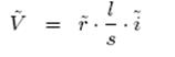 |
………………..(22) |
where ![]() is the resistivity affected by damage by means of change in volume only. Bridgeman’s law gives
is the resistivity affected by damage by means of change in volume only. Bridgeman’s law gives ![]() as:
as:
|
………………..(23) |

where, K is a coefficient which is approximately 2 for metals. If the same intensity is considered for non-damaged as well as damaged elements, the damage D may be derived from the two expressions, leading to:
 |
………………..(24) |
There are more methods available to determine damage in an RVE such as:
- Acoustic emission
- Tertiary creep stress response
- Variation of cyclic plasticity
- Ultrasonic wave propagation
- Nano-indentation, and etcetera
Effects of Damage
Damage by the creation of free surfaces of discontinuities reduces the value of many properties:
- It decreases the elasticity modulus
- It decreases the yield stress before or after hardening
- It decreases the hardness
- It increases the creep strain rate
- It decreases the ultrasonic waves velocity
- It decreases the density
- It increases the electrical resistance
Some of these effects are used to evaluate the damage by inverse methods. Furthermore, the effects on mechanical strength and stiffness are different in tension and in compression due to microcracks opening under tension and their closure under compression.
Hyperlink References further details: