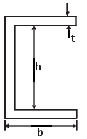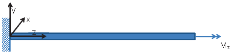
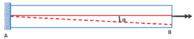
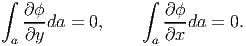
Figure 9.1: Schematic of a straight prismatic member subjected to end
torsion
In the last chapter, we studied the response of straight prismatic beams subjected to bending moments. In this chapter, we study the stresses that develop and the displacement that these members undergo when subjected to twisting moment. While in the analysis of beams subjected to bending moments we maintained some generality with the loading, the study of torsion is focused on a single loading case - one end fixed and the other end free to twist, as shown in figure 9.1. Here the double arrow indicates the twisting moment. However, we study this boundary value problem for a variety of cross sections. This analysis for torsion depends on whether the section is thick walled or thin walled as in the case of bending moments. It also depends on whether the section is open or closed. We shall discuss in detail as to when a section is closed subsequently.
Before proceeding further, we would like to point out the change in the orientation of the coordinate system, from that used in the study of the beams. This is necessitated because for some problems we would be using cylindrical polar coordinates, and want the cross section to be in the xy plane. We use cylindrical polar coordinates with this orientation so that the boundary of the cross section can be defined easily. Since, the value of displacement or stress in a material particle is independent of the coordinate system used, it is expected that the analyst pick coordinate systems that is convenient for a problem and not that which he is comfortable with. Hence, the change.
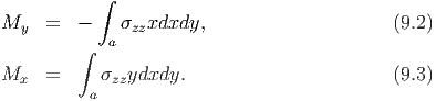
For this orientation of the coordinate system, following the same steps as discussed in detail in chapter 8, it can be shown that the torsional moment, Mz is given by,
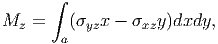 | (9.1) |
and for completeness, the other two components of the moment, which are bending moments are,
Comparing equations (9.1) with (9.2) and (9.3) it can be seen that while the bending moments are due to normal stresses, torsional moment is due to shear stresses. This is the major difference between the bending and twisting moment. While the bending moment gives raise to normal stresses predominantly, twisting moment gives raise to shear stresses predominantly.Now let us see how to classify the sections. As in case of bending, a cross section would be classified as thin walled if the thickness of the cross section is such that it is much less than the characteristic dimensions of the cross section. Typically, if the ratio of the thickness of the cross section to the length of the member is less than 0.1, the section is classified as thin. If the section is not thin, it is considered to be thick.


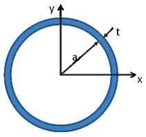
If a section when twisted can deform such that plane sections before deformation remain plane after twisting is called closed section. Sections which do not deform in the above manner are called open sections. Solid Circular cross section is an example of closed section and solid rectangular cross section is an example of open sections. Similarly, a thin walled annular cylinder (see figure 9.2) is an example of closed section and if the same annular cylinder has a longitudinal slit (see figure 9.3), it is an example of open section. All closed section allows for continuous variation of shear stresses such that it is no where zero except at the centroid of the cross section. A section which requires the shear stresses to be zero at locations apart from the centroid of the cross section, like at the corners of a rectangular cross section, is an open section. It should be pointed out that in elliptical shaped cross section also the shear stress is zero only at the centroid of the cross section but is an open section as plane sections do not remain plane after twisting. Thus, the requirement on the shear stress is just necessary but not sufficient to classify a given section as closed.
In the following section, we find the displacement field and stress field for twisting of a thick walled sections and then focus on thin walled sections.
First, we study the twisting of thick walled closed section and then thin walled
closed section. This problem we study using the displacement approach. We also
use cylindrical polar coordinates to formulate and study the problem. While the
solution that we obtain does not require that the cross section to be closed section
be circular, we shall assume this for illustration purpose, mainly to fix the
geometry of the body. Thus, we assume the body to be an right circular annular
(or solid) cylinder occupying a region in the Euclidean point space given by:  =
{(r,θ,z)|Ri ≤ r ≤ Ro, 0 ≤ θ ≤ 2π, 0 ≤ z ≤ L}, where Ri, Ro and L are constants
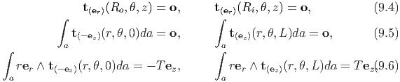
with Ri = 0 in case of solid cylinder. Since, we are interested in this body being
subjected to pure torsional moment, the traction boundary conditions are
=
{(r,θ,z)|Ri ≤ r ≤ Ro, 0 ≤ θ ≤ 2π, 0 ≤ z ≤ L}, where Ri, Ro and L are constants
with Ri = 0 in case of solid cylinder. Since, we are interested in this body being
subjected to pure torsional moment, the traction boundary conditions are
 | (9.7) |
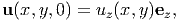
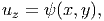
where uz denotes the z component of the displacement field and we have assumed that the surface of the body defined by z = 0 is fixed and the other surfaces are free to displace radially and circumferentially.
 (a) Schematic of deformation in the yz plane
 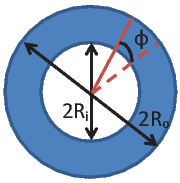 (b) Schematic of deformation in
the xy plane
(b) Schematic of deformation in
the xy plane
Since, we are going to solve the problem using the displacement approach, we have to assume the displacement field. We shall assume that plane sections normal to the axis of the member, ez remain plane and perpendicular to the axis. This means that the z component of the displacement field is only a function of z, i.e., uz = ûz(z). Further, the boundary condition (9.7) requires that uz(0) = uz(L) = 0. Consistent with these requirements, we assume that the z component of the displacement, uz = 0. We could have also assumed uz = C sin(mπz∕L), where m is an integer and C is a constant. However, it can be shown that such an assumption to satisfy balance of linear momentum would require that C = 0. Then, we shall assume that there is no radial component of the displacement, i.e., ur = 0. Since, straight radial lines before deformation remain as straight radial lines after deformation with their length unchanged, we are justified in making the assumption that ur = 0. Further, we assume that the straight line along the axis of the member remains straight but rotates by an angle θ and that the radial lines rotate by an angle ϕ as shown in the figure, 9.4 when subjected to twisting moment. Consequently, the circumferential component of the displacement, uθ = Ωrz, where Ω is called as the angle of twist per unit length. The slope of the straight line along the axis of the member located at a radial distance, r* after deformation, α = Ωr*. Similarly, the rotation undergone by radial lines in a plane defined by z = z*, where z* is a constant, is ϕ = Ωz*. Thus, the displacement field is taken as,
 | (9.8) |
It can then be verified that this displacement field satisfies the displacement boundary conditions (9.7). Then, the strain field corresponding to the displacement field (9.8) is
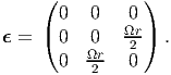 | (9.9) |
Using isotropic Hooke’s law, (7.2) the stress corresponding to the strain (9.9) is computed as
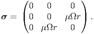 | (9.10) |
It can then be verified that the above state of stress, satisfies the static equilibrium equations in the absence of body forces, (7.6) trivially. It can also be verified that the stress given in equation (9.10) satisfies the boundary condition (9.4) trivially. For the stress state (9.10) the boundary condition (9.5) evaluates to
 | (9.11) |
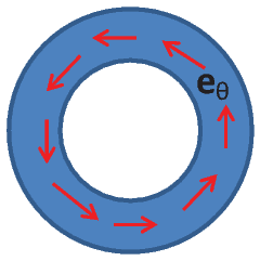
Since, the direction of eθ changes with the location as shown in figure 9.5, we write it in terms of the fixed Cartesian basis and obtain
![∫ Ro ∫ 2π
± μΩr2dr [- sin(θ)ex + cos(θ)ey]dθ = o.
Ri 0](main1190x.png) | (9.12) |
Thus, the boundary condition (9.5) holds for the stress state (9.10).
Then, using the boundary condition (9.6) we obtain the relationship between the applied torque, T and the angle of twist per unit length, Ω as,
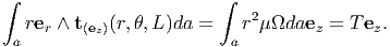 | (9.13) |
Thus,
 | (9.14) |
which for homogeneous sections reduces to
 | (9.15) |
where
 | (9.16) |
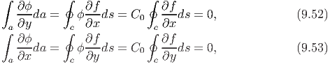
is the polar moment of inertia. Combining equations (9.10) and (9.15) we obtain
 | (9.17) |
This is called the torsion equation.
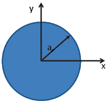
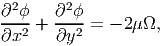
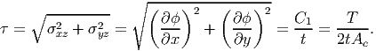
As discussed, for illustration, we consider a bar with solid circular cross section of radius R, as shown in figure 9.6. From the general expression for torsion of a thick walled close section (9.17), we find that the shear stresses in the bar is given by,
 | (9.18) |
where we have computed J = ∫ 02πdθ ∫ 0Rr3dr. Thus, we find that the shear stress varies linearly with the radial distance, as shown in figure 9.7.
Then, the angle of twist per unit length, Ω is also obtained from (9.17) as,
 | (9.19) |
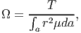
Having determined the angle of twist per unit length, the entire displacement field corresponding to an applied torque, T given by equation (9.8) is known. The same is plotted in figure 9.8.
 (a) Undeformed circular bar
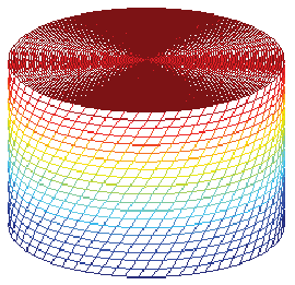 (b) Deformed circular bar
In this section, as in the previous, we consider a bar subjected to twisting moments at its ends. The bar axis is straight and the shape of the cross section is constant along the axis. The bar is assumed to have a solid cross section, i.e, a simply connected domain. A domain is said to be simply connected if any closed curve in the domain can be shrunk to a point in the domain itself, without leaving the domain. A domain which is not simply connected is said to be multiply connected. We shall analyze multiply connected domains in the next section.
Though the problem formulation does not assume any specific shape for the
cross section, the displacement and stress field obtained are cross section
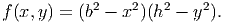
specific. Let us assume that the boundary of the cross section is defined by
a function, f(x,y) = 0. This function for a ellipse centered about the
origin and major and minor axis oriented about the ex and ey directions
would be, f(x,y) = x2∕a2 + y2∕b2 - 1. Consequently, for the body is
assumed to occupy a region in Euclidean point space, defined by =
{(x,y,z)|f(x,y) ≤ 0, 0 ≤ Z ≤ L}, where L is a constant. Here we are assuming
that the bar is a solid cross section with the cross section having only one
surface, f(x,y) = 0 denoted by ∂ . To be more precise, the cross section is
simply connected. Since, we are interested in the case where in the bar is
subjected to pure end torsional moment, the traction boundary conditions are:
. To be more precise, the cross section is
simply connected. Since, we are interested in the case where in the bar is
subjected to pure end torsional moment, the traction boundary conditions are:
![∂f ∂f
--[∂y-ex --∂xey]--
en = ∘ (---)---(---)2-,
∂f- 2 + ∂f
∂x ∂y](main1204x.png) | (9.25) |
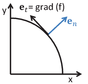
and T is a constant. Here en is obtained such that it is in the xy plane,
perpendicular to grad(f) and is a unit vector. Recognize that grad(f) gives the
tangent vector to the cross section for any point in ∂. The orientation of en and
grad(f) is as shown in figure 9.9. Further, since one end of this body is assumed
to be fixed against twisting but free to displace axially and the other end free to
displace in all directions, the displacement boundary conditions for this problem
is,
 | (9.26) |
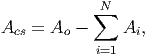
where uz is any function of x and y. Here we have assumed that the surface of the body defined by z = 0 is fixed against twisting but free to displace axially and the other surfaces are free to displace in all directions.
In a solid cross section, as a result of a twist, each cross section undergoes a rotational displacement about the z axis. For any two cross sections the relative angle of rotation is called the angle of twist between the two sections. Let Δβ be the angle of twist for two cross sections at distance Δz and Ω be the angle of twist per unit length of the bar, then
 | (9.27) |
Since the conditions are same for all cross sections, the above equation applies to any two cross sections at a distance Δz along the bar length. Thus, Ω is a constant along the bar length. Also, since at z = 0, β = 0, by virtue of the surface defined by z = 0 being fixed against rotation, the angle of twist, β for a cross sections at distance z from the surface defined by z = 0 is
 | (9.28) |
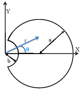
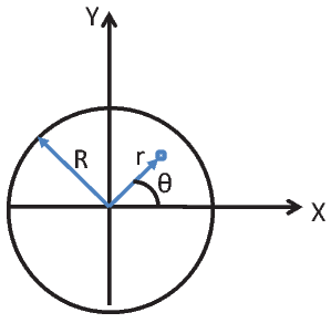
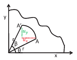
Consider a cross section at a distance z from the fixed end. In that section consider a point A with coordinates (x,y,z). Assuming the origin of the coordinate system to be located at the axis of twisting, let r denote the radial distance of the point A from the origin and let θ denote the angle that this radial line makes with the ex, as shown in the figure 9.10. Let A move to A′ due to twisting of the bar, as shown in the figure 9.10. The arc length AA′ would be equal to rβ, where β is the angle of twist at the cross section and is related to the angle of twist per unit length through (9.28). Hence, the arc length AA′ would be,
 | (9.29) |
Since, the angle of twist β is small, we approximate the secant length, i.e., the length of the straight line between AA′ with its arc length. Consequently, the x component of the displacement of A is given by,
 | (9.30) |
where we have used (9.29) and the relation that y = r sin(θ). Similarly, the y component of the displacement of A is,
 | (9.31) |
where as before we used (9.29) and the relation x = r cos(θ). Since, there is no restraint against displacement along ez direction at any section, all cross sections is assumed to undergo the same displacement along the z direction and hence
 | (9.32) |
where ψ is a function of x and y only. That is, we have assumed that the z component of the displacement is independent of the axial location of the section. Presence of this z component of the displacement is the characteristic of open sections. It is due to this z component of the displacement the plane section distorts and is said to warp. Consequently, ψ is called Saint-Venant’s warping function. Thus, the displacement field for a bar subjected to twisting moments at the end and is free to warp is given by,
 | (9.33) |
It can be easily verified that the above displacement field (9.33) satisfies the displacement boundary condition (9.26).
Substituting equation (9.33) in the strain-displacement equation (7.1), the Cartesian components of the strain are computed to be
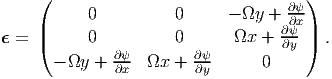 | (9.34) |
For this state of strain, the corresponding Cartesian components of the stress are obtained from Hooke’s law (7.2) as
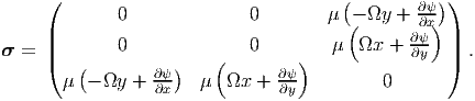 | (9.35) |
For this stress state, (9.35) to be possible in a body in static equilibrium, without any body force acting on it, it should satisfy the balance of linear momentum equations (7.6) which requires that,
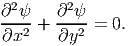 | (9.36) |
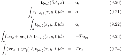
Now, we have to find ψ such that equation (9.36) holds along with the prescribed traction boundary conditions (9.20) through (9.24).
Boundary condition (9.20) requires
![[ ] [ ]
μ - Ωy + ∂ψ- ∂f-- μ Ωx + ∂-ψ ∂f- = 0,
∂x ∂y ∂y ∂x](main1218x.png) | (9.37) |
for (x,y) ∈ ∂. Both the boundary conditions (9.21) and (9.22) yield the
following restriction on ψ,
![∫ [ ] ∫ [ ]
∂ψ- ∂-ψ
μ - Ωy + ∂x da = 0, μ Ωx + ∂y da = 0,
a a](main1219x.png) | (9.38) |
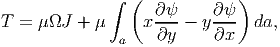
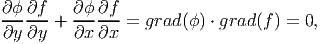
On assuming that the bar is homogeneous and appealing to Green’s theorem (section 2.9.3), equation (9.38) reduces to,
where (xc,yc) is the coordinates of the centroid of the cross section. On assuming that the axis of twisting coincides with the centroid and further requiring that the origin of the coordinate system coincide with the centroid of the cross section, equations (9.39) and (9.40) requires,
 | (9.41) |
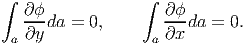
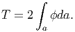
Finally, the boundary conditions (9.23) and (9.24) require that
 | (9.42) |
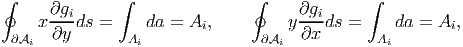
Recognizing that ∫ a(x2 + y2)da = J, polar moment of inertia equation (9.42) can be simplified as,
 | (9.43) |
where we have used the assumption already made that the bar is homogeneous.
For many cross sections, ∫
a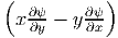 da < 0. Thus, the torsional
stiffness1
which would be μJ, in the absence of warping (i.e., ψ = 0), decreases
due to warping (i.e., when ψ ≠ 0). Hence, warping is said to decrease
the torsional stiffness of the cross section. Equation (9.43) is used find
Ω.
da < 0. Thus, the torsional
stiffness1
which would be μJ, in the absence of warping (i.e., ψ = 0), decreases
due to warping (i.e., when ψ ≠ 0). Hence, warping is said to decrease
the torsional stiffness of the cross section. Equation (9.43) is used find
Ω.
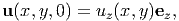
Experience has shown that it is difficult to find ψ that satisfies the governing equation (9.36) along with the boundary conditions (9.37) and (9.41). Hence, we recast the problem using Prandtl stress function.
Defining a differentiable function, ϕ =  (x,y) called the Prandtl stress
function, we relate the components of the stress to this stress function
as,
(x,y) called the Prandtl stress
function, we relate the components of the stress to this stress function
as,
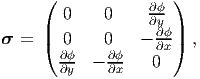 | (9.44) |
so that the equilibrium equations (7.6) are satisfied for any choice of ϕ.
Now, one can proceed in one of two ways. Follow the standard approach and find the strain corresponding to the stress state (9.44), substitute the same in the compatibility conditions and find the governing equation that ϕ should satisfy. Here we obtain the same governing equation through an alternate approach.
Equating the stress states (9.35) and (9.44) as it represents for the same boundary value problem, we obtain
Differentiating equation (9.45) with respect to y and equation (9.46) with respect to x and adding the resulting equations, we obtain
 | (9.47) |
where we have made use of the requirement that  =
=  . By virtue of the
stress function being smooth enough so that
. By virtue of the
stress function being smooth enough so that  =
=  , the governing equation
for ψ (9.36) is trivially satisfied.
, the governing equation
for ψ (9.36) is trivially satisfied.
The boundary condition given in equation (9.37) in terms of the warping function, ψ is rewritten in terms of the Prandtl stress function, ϕ using equations (9.45) and (9.46) as,
 | (9.48) |
for (x,y) ∈ ∂. Since, grad(f) ≠ o and its direction changes with the location on
the boundary of the cross section, grad(ϕ) = o on the boundary of the cross
section. This implies that
 | (9.49) |
where C0 is a constant. Since, the stress and displacement fields depend only in the derivative of the stress potential and not its value at a location, it suffices to find this stress function up to a constant2 . Therefore, we arbitrarily set C0 = 0, understanding that it can take any value and that the stress and displacement field would not change because of this. Hence, equation (9.49) reduces to requiring,
 | (9.50) |
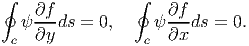
The boundary condition (9.21) and (9.22) for the stress state (9.44) require
 | (9.51) |
Appealing to Green’s theorem for simply connected domains, the above equation (9.51) reduces to
where we have used (9.49) and the fact that ∮ c ds = 0 and ∮
c
ds = 0 and ∮
c ds = 0 for
closed curves.
ds = 0 for
closed curves.
Finally, the boundary conditions (9.23) and (9.24) for the stress state (9.44) yields,
![∫ [ ]
- x∂-ϕ + y∂-ϕ da = T.
a ∂x ∂y](main1240x.png) | (9.54) |
Noting that
where we have used the Green’s theorem for simply connected domain and equation (9.50). Substituting the above equations in (9.54) we obtain,
 | (9.57) |
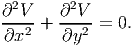
Thus, we have to find ϕ such that the governing equation (9.47) has to hold along with the boundary condition (9.50). Then, we use equation (9.57) to find the torsional moment required to realize a given angle of twist per unit length Ω.
The governing equation (9.47) along with the boundary condition (9.50) and (9.57) is identical with those governing the static deflection under uniform pressure of an elastic membrane in the same shape as that of the member subjected to torsion. This fact creates an analogy between the torsion problem and elastic membrane under uniform pressure. This analogy is exploited to get the qualitative features that the stress function should posses and this aids in developing approximate solutions. Obtaining the governing equation for the static deflection of an elastic membrane under uniform pressure and showing that it is identical to (9.47) is beyond the scope of this lecture notes. One may refer Sadd [4] for the same.
In the following three sections, we apply the above general framework to solve problems of bars with specific cross section shapes subjected to end torsion.
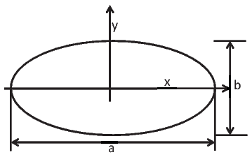
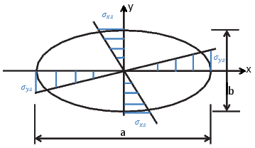
The first cross section shape that we consider is that of an ellipse. That is we study a bar with elliptical cross section, whose boundary is defined by the function,
 | (9.58) |
where a and b are constants and we have assumed that the major and minor axis of the ellipse coincides with the coordinate basis, as shown in the figure 9.11.
Choosing the Prandtl stress function to be,
![[ ]
x2 y2
ϕ = C -2-+ -2-- 1 ,
a b](main1245x.png) | (9.59) |
where C is a constant, we find that it satisfies the boundary condition (9.50). Substituting the stress function, (9.59) in the equation (9.47) we obtain
 | (9.60) |
Using (9.59) and (9.60) in (9.57), twisting moment is obtained as
 | (9.61) |
Corresponding to the stress function (9.59) the shear stresses are computed to be

The resultant shear stress in the xy plane is given by,
 | (9.63) |
It is clear from equation (9.63) that the extremum shear stress occurs at (0, 0) or the boundary of the cross section. It can be seen that at (0, 0) minimum shear stress occurs, as τ = 0 at this location. At the boundary the extremum shear stresses would occur at (0,±b) and (±a, 0). Thus, the extremum shear stresses are τext = 2T∕(πab2) at (0,±b) and τ ext = 2T∕(πba2) at (±a, 0). If a > b, then the maximum shear stress in the elliptical cross section is,
 | (9.64) |
Substituting (9.59) in equations (9.45) and (9.46) and rearranging we obtain
![[ ]
∂ψ- 2C-- ∂ψ- 2C--
∂x = Ωy + μb2y, ∂y = - Ωx + μa2 x .](main1252x.png) | (9.65) |
Solving the differential equations (9.65) we obtain
 | (9.66) |
where D0 is a constant. Since, there is no rigid body translation, we require that ψ(0, 0) = 0. Hence, D0 = 0. Thus, we find that the section warps into a diagonally symmetric surface as shown in figure 9.13.
Rearranging the equation (9.61) we can get Ω as a function of torque, T as
![T[a2 + b2]
Ω = -----3-3--
μπa b](main1254x.png) | (9.67) |
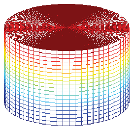
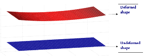
The entire displacement field, (9.33) for a bar with elliptical cross section is now known that we have found the warping function (9.66). The deformation of a bar with the elliptical cross section computed using this displacement field is shown in figure 9.14.
 (a) Undeformed elliptical bar
  (b) Deformed elliptical bar
Before concluding this section let us see the error that would have been made if one analyzes the elliptical section as a closed section. The polar moment of inertia for the elliptical section could be computed and shown to be J = πab(a2 + b2)∕4. Then, the angle of twist per unit length computed from (9.17) would be,
![Ω = -----4T------.
cl μ πab[a2 + b2]](main1258x.png) | (9.68) |
The ratio of Ωcl∕Ω, computed from equations (9.68) and (9.67) is
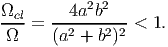 | (9.69) |
Thus, for a given torque open section twists more.
Next, we examine the shear stresses. If one uses (9.17) to compute the shear stresses, they would erroneously conclude that the maximum shear stress occurs at (±a, 0), by virtue of these points being farthest from the center of twist and the value of this maximum shear stress would be,
![4T
τcmlax = ----2---2--
πb[a + b ]](main1260x.png) | (9.70) |
Comparing equations (9.64) and (9.70) we find that
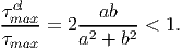 | (9.71) |
Thus, closed section underestimates the stresses in the bar.
Hence, from both strength and serviceability point of view assuming the elliptical cross section to be closed would result in an unsafe design.
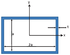
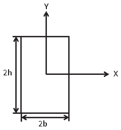
Next, we assume that the bar has a rectangular cross section of width 2b and depth 2h, as shown in figure 9.15. For this section the boundary is defined by the function,
 | (9.72) |
It can be verified that choosing the Prandtl stress function, ϕ as Cf(x,y) would not satisfy the governing equation (9.47). Hence, we assume a stress function of the form,
![2 2
ϕ = μ Ω[V (x,y) + b - x ],](main1264x.png) | (9.73) |
where V is a function of (x,y).
Substituting equation (9.73) in equation (9.47) and simplifying we obtain,
 | (9.74) |
Then, the boundary condition (9.50) requires that
 | (9.75) |
Thus, we need to solve the differential equation (9.74) subject to the boundary condition (9.75).
Towards this, we seek solution of the form
 | (9.76) |
where V x is a function of x and V y is a function of y alone. Substituting the assumed special form for V , (9.76) in equation (9.74) and simplifying we obtain,
 | (9.77) |
where k is any constant. Recognize that the left hand side of the equation is a function of x alone and the right hand side is a function of y alone. Hence, for these functions to be same, they have to be a constant. Solving the second order ordinary differential equations (9.77) we obtain,
 | (9.78) |
Consistent with the boundary condition (9.75), we expect the functions V x and V y to be even functions, i.e., V x(-x) = V x(x) and V y(-y) = V y(y). Hence,
 | (9.79) |
Substituting (9.79) in the equation (9.78) and the result into equation (9.76) we obtain,
 | (9.80) |
where E is some arbitrary constant. The equation (9.80) on applying the boundary condition (9.75a), i.e., V (±b,y) = 0 yields that
 | (9.81) |
where n is any integer. Since, the governing equation for V , (9.74) is a Laplace equation, it is a linear equation. Consequently, if two functions satisfy the given equation (9.74) then a linear combination of these functions also satisfies the Laplace equation. So the solution (9.80) can be written as,
 | (9.82) |
where En’s are constant. Substituting (9.82) in the boundary condition (9.75b), i.e., V (x,±h) = x2 - h2 we obtain,
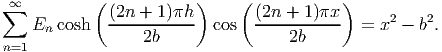 | (9.83) |
Now, we have to find the constants En such that for -b ≤ x ≤ b, a linear combination of cosines approximates the quadratic function on the right hand side of equation (9.83). Using the standard techniques in fourier analysis we obtain,
![( ) ∫ b ( )
En cosh (2n-+-1)πh- = [x2 - b2]cos (2n-+-1-)πx- .
2b -b 2b](main1275x.png) | (9.84) |
Integrating the above equation and rearranging, we obtain
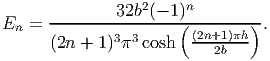 | (9.85) |
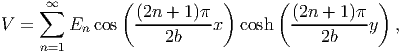
Substituting equation (9.85) in (9.82) and the resulting equation in (9.73), we obtain
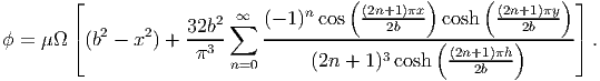 | (9.86) |
Having found the stress function, we are now in a position to find the shear stresses and the warping function. First, we compute the stresses as,
![∂ϕ
σxz = ---
∂y ( ( ) [ ] ( ) )
2 { ∞ (- 1)ncos (2n+1)πx- (2n+1)π- sinh (2n+1-)πy }
= μΩ 32b-- ∑ --------------2b--------2b(--------)----2b---- ,
π3 ( 3 (2n+1)πh- )
n=0 (2n + 1) cosh 2b](main1278x.png) | (9.87) |
![σyz = - ∂ϕ-
(∂x ( ) [ ] ( ))
{ 2∑∞ (- 1)nsin (2n+1)πx- (2n+1)π cosh (2n+1)πy }
= μΩ 2x + 32b-- --------------2b--------2(b-------)----2b---- .
( π3 (2n + 1)3cosh (2n+1)πh- )
n=0 2b](main1279x.png) | (9.88) |
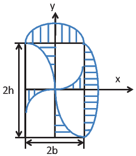
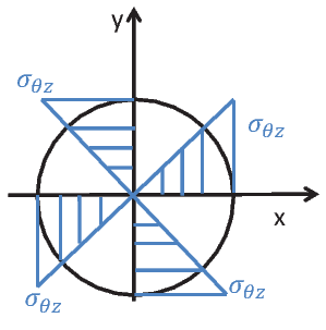
Figure 9.16 schematically shows the shear stress distribution in a rectangular cross section along the sides of the rectangle and along the lines x = 0 and y = 0. The shear stress is maximum on the boundary and zero at the center of the rectangle. The maximum shear stress occurs at the middle of the long side and is given by,
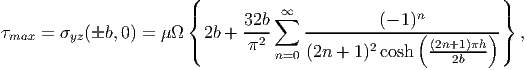 | (9.89) |
where we have assumed that h ≥ b.
Substituting (9.87) in equation (9.45) and solving the first order ordinary differential equation for ψ we obtain
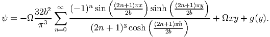 | (9.90) |
Substituting equations (9.88) and (9.90) in equation (9.46) and solving the first order ordinary differential equation for g we obtain g(y) = D0, a constant. Since, the bar does not move as a rigid body, we want ψ(0, 0) = 0. Hence, D0 = 0. Consequently, the warping function is,
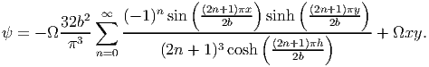 | (9.91) |
Figure 9.17 plots the warped rectangular section.
Substituting (9.87) and (9.88) in equation (9.57) we can relate the applied torque, T to the realized angle of twist per unit length, Ω as
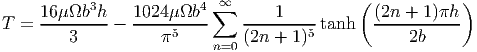 | (9.92) |
This relation is expressed as
 | (9.93) |
where C1 is a non-dimensional parameter which depends on h∕b. In the same spirit, the maximum shear stress, (9.89) could be related to the applied torque as,
 | (9.94) |
where C2 is another non-dimensional parameter which depends on h∕b. Values of C1 and C2 for various h∕b ratios are tabulated in table 9.1.
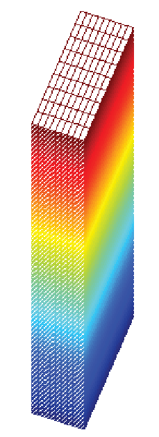 (a) Undeformed rectangular bar
 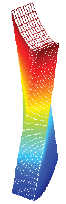 (b) Deformed rectangular bar
| h∕b | C1 | C2 |
| 1 | 0.141 | 4.80 |
| 1.5 | 0.196 | 4.33 |
| 2.0 | 0.229 | 4.06 |
| 3.0 | 0.263 | 3.74 |
| 4.0 | 0.281 | 3.54 |
| 6 | 0.299 | 3.34 |
| 10 | 0.312 | 3.21 |
| ∞ | 0.333 | 3.00 |
Thus, for thin rectangular sections, when h∕b tends to ∞,
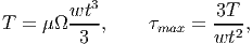 | (9.95) |
where we have assumed the section to have a thickness, t = 2b and depth, w = 2h. It should be mentioned that irrespective of the orientation of the thin rectangular section, the equation (9.95) remains the same. This is because of the requirement that h ≥ b. Physically, irrespective of the orientation of the section, the torsion is resisted by the spatial variation of the shear stresses through the thickness of the section as shown in figure 9.19.
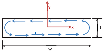 (a) Thin rectangular section oriented along x direction
 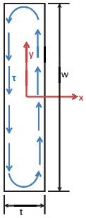 (b) Thin rectangular
section oriented along y
direction
(b) Thin rectangular
section oriented along y
direction
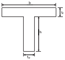
Here we study the problem of end torsion of a bar whose cross section is narrow and has small curvature such as those shown in figure 9.20. Such sections are usually made of hot rolled steel and hence are called rolled sections. Since, the shape across the thickness is similar to that of the thin rectangular section, excepting at the bent corners, it is assumed that the solution obtained for thin rectangular section holds. In order for the corners not to change the displacement and stress field from that obtained for a thin rectangular section, it is required that the radius of curvature of these corners be large.
 (a) Angle section
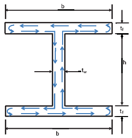 (b) I section
Thus, for the angle section shown in figure 9.20a, the torque required to realize a given angle of twist per unit length and the maximum shear stress in the section is obtained from (9.95) as
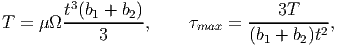 | (9.96) |
where we have treated the entire angle without the 90 degree bend, as a thin walled rectangular section. In order for the above equations to be reasonable, (b1 + b2)∕t > 10 and the radius of the curvature of the bent corner large.
Similarly, for the I section shown in figure 9.20b, the torque required to realize a given angle of twist per unit length and the maximum shear stress in the section is obtained from (9.95) as
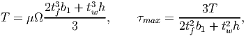 | (9.97) |
where the torsional stiffness due to each of the three plates - the two flange plates and the web plate - is summed algebraically. This is justified because the shear stress distribution in each of these plates is similar to that of a thin rectangular section subjected to torsion, as indicated in the figure 9.20b. However, comparison of this solution with the exact result for this geometry is beyond the scope of this notes.
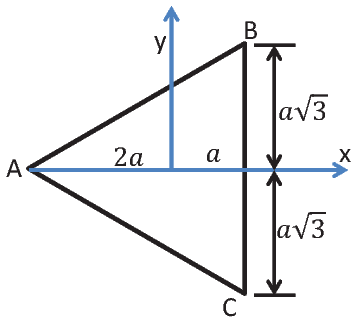
Finally, we consider the torsion of a cylinder with equilateral triangle cross section, as shown in figure 9.21. The boundary of this section is defined by,
![√ -- √ --
f(x,y ) = [x - 3y + 2a][x + 3y + 2a][x - a] = 0,](main1298x.png) | (9.98) |
where a is a constant and we have simply used the product form of each boundary line equation. Assuming that the Prandtl stress function to be of the form,
![√ -- √ --
ϕ = K [x - 3y + 2a][x + 3y + 2a][x - a],](main1299x.png) | (9.99) |
so that the boundary condition (9.50) is satisfied. It can then be verified that the potential given in equation (9.99) satisfies (9.47) if
 | (9.100) |
Substituting equation (9.99) in (9.57) and using (9.100) we obtain the torque to be
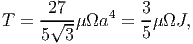 | (9.101) |
where the polar moment of inertia for the equilateral triangle section, J =
3 a4.
a4.
The shear stresses given in equation (9.44) evaluates to
on using equations (9.99) and (9.100). The magnitude of the shear stress at any point is given by,
 | (9.104) |
Since, for torsion the maximum shear stress occurs at the boundary of the cross section, we investigate the same at the three boundary lines. We begin with the boundary x = a. It is evident from (9.102) that on this boundary σxz = 0. Then, it follows from (9.103) that σyz is maximum at y = 0 and this maximum value is 3aμΩ∕2. It can be seen that on the other two boundaries too the maximum shear stress, τmax = 3aμΩ∕2.
Substituting (9.99) in equations (9.45) and (9.46) and solving the first order differential equations, we obtain the warping displacement as,
![ψ = -Ω-y[3x2 - y2],
6a](main1305x.png) | (9.105) |
on using the condition that the origin of the coordinate system does not get displaced; a requirement to prevent the body from displacing as a rigid body.
In this section, as in the previous, we consider a bar subjected to twisting moments at its ends. The bar axis is straight and the shape of the cross section is constant along the axis. The bar is assumed to have a hollow cross section, i.e, a multiply connected domain. That is any closed curves in the cross section cannot be shrunk to a point in the domain itself without leaving the domain.
Let us assume that the boundary of the cross section is defined by a
function, f(x,y) = 0, the set of points constituting this boundary by
∂o, and the enclosed area by Ao. The boundary of the ith void in the
interior of the cross section is defined by the function gi(x,y) = 0, the set of
points constituting this boundary of the ith void by ∂
i and the area
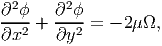
enclosed by the void, Ai. Thus, the area of the cross section, Acs is given
by
 | (9.106) |
where we have assumed that there are N voids.
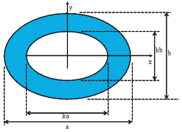
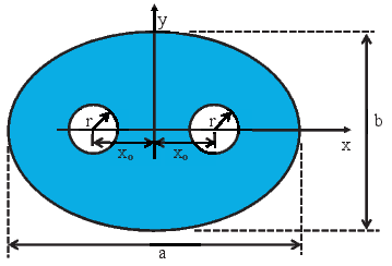
Thus, for the cross section shown in figure 9.22, with the boundary of the cross
section in the form of an ellipse centered about origin and oriented such that the
major and minor axis coincides with the ex and ey directions respectively and
having two circular shaped voids of radius, r centered at (±xo, 0), the functions
f(x,y) and gi(x,y) would be: f(x,y) = x2∕a2 + y2∕b2 - 1, g
1(x,y) =
(x - xo)2 + y2 - r2 and g
2(x,y) = (x + xo)2 + y2 - r2. Consequently, this body is
assumed to occupy a region in Euclidean point space, defined by =
{(x,y,z)|f(x,y) ≤ 0, 0 ≤ Z ≤ L}-{(x,y,z)|f(x,y) ≤ 0, 0 ≤ Z ≤ L}-
{(x,y,z)|f(x,y) ≤ 0, 0 ≤ Z ≤ L}-{(x,y,z)|g1(x,y) ≤ 0, 0 ≤ Z ≤ L}-
{(x,y,z)|f(x,y) ≤ 0, 0 ≤ Z ≤ L}-{(x,y,z)|g2(x,y) ≤ 0, 0 ≤ Z ≤ L}, where L is
a constant.
Since, we are interested in the case where in the bar is subjected to pure end torsional moment, the traction boundary conditions are:
where
![[∂∂fyex - ∂∂fxey] [∂g∂iy ex - ∂∂gxiey]
en = ∘----------(--)--, emi = ∘----------(---)-,
(∂f)2 + ∂f 2 (∂gi)2 + ∂gi 2
∂x ∂y ∂x ∂y](main1309x.png) | (9.113) |
and T is a constant. Here en is obtained such that it is in the xy plane,
perpendicular to grad(f) and is a unit vector. Similarly, emi is obtained such that
it is in the xy plane, perpendicular to grad(gi) and is a unit vector. Recognize
that grad(f) gives the tangent vector to the cross section for any point in ∂o
and grad(gi) is the tangent vector to the cross section at any point in
∂i. Further, since one end of this body is assumed to be fixed against
twisting but free to displace axially and the other end free to displace in
all directions, the displacement boundary conditions for this problem
is,
 | (9.114) |
where uz is any function of x and y. Here we have assumed that the surface of the body defined by z = 0 is fixed against twisting but free to displace axially and the other surfaces are free to displace in all directions.
Thus, we find that the boundary value problem is similar to that in the
previous section (section 9.3) except for the additional boundary condition
(9.108). Hence, we assume that the stress is as given in equation (9.44), in terms
of the Prandtl stress function, ϕ =  (x,y). Following the standard procedure, as
outlined in section 9.3, it can be shown that the stress function should
satisfy,
(x,y). Following the standard procedure, as
outlined in section 9.3, it can be shown that the stress function should
satisfy,
 | (9.115) |
where μ is the shear modulus, and Ω is the angle of twist per unit length.
For the assumed stress state, (9.44), the boundary condition (9.107) requires
that grad(ϕ) ⋅ grad(f) = 0 on ∂o. Thus,
 | (9.116) |
where C0 is a constant. As before, since, the stress and displacement fields depend only in the derivative of the stress potential and not its value at a location, it suffices to find this stress function up to a constant. Therefore, we arbitrarily set C0 = 0, understanding that it can take any value and that the stress and displacement field would not change because of this. Hence, equation (9.116) reduces to requiring,
 | (9.117) |
The boundary condition (9.108) requires that grad(ϕ) ⋅ grad(gi) = 0 on ∂i.
Hence,
 | (9.118) |
where Ci’s are constants. Though ϕ is a constant over all free surfaces, the value
of this constant can differ between distinct free surfaces, i.e., ∂i. Also, recognize
that these constants cannot be set to zero, as we have already set C0 =
0.
The boundary condition (9.109) and (9.110) for the stress state (9.44) require
 | (9.119) |
Appealing to Green’s theorem for multiply connected domains, (2.278) and (2.279), the above equation (9.119) reduces to
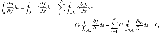 | (9.120) |
 | (9.121) |
 ograd(f)ds
= 0, ∮
∂igrad(gi)ds = 0.
ograd(f)ds
= 0, ∮
∂igrad(gi)ds = 0.
Finally, the boundary conditions (9.111) and (9.112) for the stress state (9.44) yields,
![∫ [ ∂ ϕ ∂ ϕ]
- x--- + y--- da = T.
a ∂x ∂y](main1319x.png) | (9.122) |
Noting that
![[ ]
∫ ∂ ϕ ∫ ∂(x ϕ) ∮ ∂f N∑ ∮ ∂gi ∫
x--- = ------ - ϕ da = xϕ ---ds- xϕ ---ds - ϕda
a ∂x a ∂x ∂Ao ∂y i=1 ∂Ai ∂y a
∑N ∮ ∫ ∑N ∫
= - Ci x∂gids - ϕda = - CiAi - ϕda,
i=1 ∂Ai ∂y a i=1 a](main1320x.png) | (9.123) |
![∫ ∂ϕ ∫ [∂(yϕ ) ] ∮ ∂f ∑N ∮ ∂gi ∫
y--- = ------- ϕ da = yϕ---ds - yϕ----ds - ϕda
a ∂y a ∂y ∂Ao ∂x i=1 ∂Ai ∂x a
∑N ∮ ∫ ∑N ∫
= - C y∂gids - ϕda = - C A - ϕda,
i ∂Ai ∂x a i i a
i=1 i=1](main1321x.png) | (9.124) |
 | (9.125) |
where Ai is the area enclosed by the void.
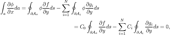
Substituting the above equations (9.123) and (9.124) in (9.122) we obtain,
 | (9.126) |
Thus, we have to find ϕ such that the governing equation (9.115) has to hold along with the boundary conditions (9.117) and (9.118). Then, we use equation (9.126) to find the torsional moment required to realize a given angle of twist per unit length, Ω.
Here we study the torsion of a bar with a hollow elliptical section as shown in figure 9.23 where the inner boundary is a scaled ellipse similar to that of the outer boundary. Since, the inner ellipse is a scaled outer ellipse, the Prandtl stress function obtained for solid ellipse cross section in section 9.3.1 is a constant at the inner surface. Hence, the boundary condition (9.118) holds and therefore this stress function
![[ ]
--a2b2- x2- y2-
ϕ = μΩ a2 + b2 a2 + b2 - 1 ,](main1325x.png) | (9.127) |
is a solution to this boundary value problem of twisting of a hollow elliptical bar. Now, the constant C1, the value of ϕ at the inner boundary is obtained as,
![--a2b2- [ 2 ]
C1 = μΩ a2 + b2 k - 1 .](main1326x.png) | (9.128) |
Using (9.127) and (9.128) in (9.126), twisting moment is obtained as
![3 3
T = μΩ π--a-b--[1 - k4].
a2 + b2](main1327x.png) | (9.129) |
Since, the stress function is same as in the case of a solid elliptical section, the stress distribution is also identical as before. Therefore, the maximum shear stress occurs at x = 0, y = ±b and is given by,
 | (9.130) |
Before concluding this section we observe that this solution scheme can be applied to other cross sections whose inner boundary coincides with a contour line of the stress function in the corresponding solid section problem.
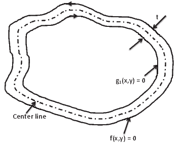
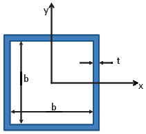
In this section, we seek approximate solution to the case when, the bar, in
the form of a thin walled tube is subjected to end torsion. We do not
assume that the cross section of the tube to be of any particular shape.
While we assume that the thickness of the cross section, t is small, we
do not assume that it is uniform. Let the boundary of the cross section
be defined by a function, f(x,y) = 0, the set of points constituting this
boundary be denoted by ∂o, and the enclosed area by Ao. The boundary in
the interior of the cross section is defined by the function g1(x,y) = 0,
the set of points constituting this boundary is denoted by ∂i and the
area enclosed by, Ai. Then the area of the cross section is Acs = Ao -
Ai.
In order to satisfy the requirement that the lateral surface is taction free, boundary conditions (9.107) and (9.108), the stress function has to be zero at the outer surface (9.117) and should be a constant at the inner surface (9.118). Hence, we assume that the stress function varies linearly through the thickness of the section. This assumption would be reasonable given that the thickness of the section is small. Thus,
 | (9.131) |
where C1 is a constant, the value of ϕ at the inner surface, ro is the radial distance of the outer boundary from the centroid of the cross section, r is the radial distance of any point in the cross section. If ri is the radial distance of the inner boundary from the centroid of the cross section, then t = ro - ri.
For the warping displacement, ψ to be single valued in the thin walled tube shown in figure 9.24,
 | (9.132) |
Substituting equations (9.45) and (9.46) in the above equation,
![∮ [ ] ∮ [ ]
1-∂ϕ- 1-∂ϕ-
∂A μ ∂y + Ωy dx - ∂A μ ∂x + Ωx dy = 0.
i i](main1332x.png) | (9.133) |
Using Green’s theorem (2.271) we find that
 | (9.134) |
Since, the stress function is assumed to vary linearly over the domain, grad(ϕ) = -C1∕ter, where er is a unit vector normal to the boundary of the cross section. Consequently,
 | (9.135) |
Substituting equations (9.134) and (9.135) in (9.133) we obtain
 | (9.136) |
Since, ϕ varies linearly through the thickness of the cross section, using trapezoidal rule for integration we find that
 | (9.137) |
where A is the area of the cross section. Here it should be pointed out that trapezoidal rule for integration gives the exact value when the variation is linear. Now, substituting equation (9.137) in (9.126) we obtain the torque to be,
![[ A ]
T = C1A + 2C1Ai = 2C1 Ai + -- = 2C1Ac,
2](main1337x.png) | (9.138) |
where Ac is the area enclosed by the centerline of the cross section. As a consequence of the section being thin walled, Ai ≈ Ac. Therefore, from equations (9.136) and (9.138) we obtain,
 | (9.139) |
Here it should be recollected that the thickness of the section can vary along the circumference of the cross section.
Finally, we estimate the shear stress in the cross section. Since, the shear stress in the cross section is equal to the magnitude of grad(ϕ), we obtain
 | (9.140) |
Thus, τt is constant throughout the section.
In this chapter, we obtained the stress and displacement fields in a straight, prismatic bar subjected to end twisting moments. For the case of thick walled closed sections and thin walled sections of any shape, we obtained an expression relating the torque with the angle of twist per unit length and the shear stress with the torque. However, for thick walled open sections, a procedure was outlined to obtain the stress and displacement fields and the same illustrated for elliptical, rectangular and triangular shaped cross sections. In all these cases, the section was assumed to be free to warp, so that no warping stresses develop. Generalization for the case when warping is restrained, is not straight forward and is beyond the scope of this lecture notes.
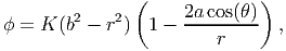 |
where K is a constant. If the stress function is admissible,
![[ ]
-----b2----
τshaft = μΩa 4a2 cos2(θ) - 1 , τkeyway = μ Ω[2a cos(θ) - b],](main1348x.png) |
where Ω is the angle of twist per unit length and μ is the shear modulus.
![[ 2 ]
ψ = - μΩ- x2 + y2 - 2ax + -2b-ax--- b2 ,
2 x2 + y2](main1349x.png) |
where x and y are the coordinates of a typical point in the cross section.
Comment on which of these sections is economical.
![∫ [ ∂ψ ] ∮ ∂f
μ - Ωy + --- da = - μΩycA + ψ∘-------∂y-------ds = 0, (9.39)
a ∂x c (∂f)2 (∂f)2
∂x + ∂y
∫ [ ] ∮ ∂f
μ Ωx + ∂ψ- da = μΩx A - ψ∘-------∂x-------ds = 0, (9.40)
a ∂y c c ( )2 ( )2
∂∂fx + ∂∂fy](main1220x.png)
![[ ]
∂ϕ ∂ψ
--- = μ - Ωy + --- , (9.45)
∂y [ ∂x ]
∂ϕ- ∂ψ-
∂x = - μ Ωx + ∂y . (9.46)](main1227x.png)
![∫ ∫ [ ] ∮ ∫ ∫
∂ϕ ∂(xϕ) ∂f
x ---= ------- ϕ da = xϕ ---ds - ϕda = - ϕda, (9.55)
∫a ∂x ∫a[ ∂x ] ∮c ∂y ∫a ∫ a
∂ϕ- ∂(yϕ-) ∂f-
a y∂y = a ∂y - ϕ da = cyϕ ∂x ds - aϕda = - aϕda, (9.56)](main1241x.png)

![μΩ-
σxz = a [x - a]y, (9.102)
μΩ
σyz = ---[x2 + 2ax - y2], (9.103)
2a](main1303x.png)