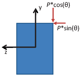
Figure 8.1: Schematic of a beam
In this chapter, we formulate and study the bending of straight and prismatic beams. First we study the bending of these beams when the loading is in the plane of symmetry of the beams cross section. Here we derive again the strength of materials solution and compare it with the solution obtained from two dimensional elasticity formulation for two loading cases, namely pure bending of a beam and uniform loading of a simply supported beam. Then, we study the bending of beams when the loading does not pass through the plane of symmetry. We do this by assuming the loading causes only bending and no torsion. We will then show that for this to happen the load should be applied at a point called the shear center of the cross-section. We conclude by presenting a method to compute this shear center.
Before proceeding further, let us begin by understanding what a beam is. A
beam is a structural member whose length along one direction, called the
longitudinal axis, is larger than its dimensions on the plane perpendicular to it
and is subjected to only transverse loads (i.e., the loads acting perpendicular to
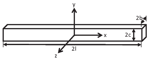
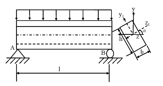
the longitudinal axis). A typical beam with rectangular cross section is shown in
figure 8.1. Thus, this beam occupies the points in the Euclidean point space
defined by  = {(x,y,z)|- l ≤ x ≤ l,-c ≤ y ≤ c,-b ≤ z ≤ b} where l, c and b
are constants, such that l > c ≥ b with l∕c typically in the range 10 to
20.
= {(x,y,z)|- l ≤ x ≤ l,-c ≤ y ≤ c,-b ≤ z ≤ b} where l, c and b
are constants, such that l > c ≥ b with l∕c typically in the range 10 to
20.
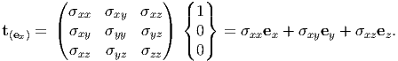
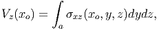
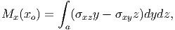
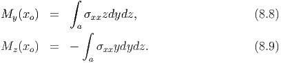
Next let us understand which moment is a bending moment and how it is related to the components of the stress. The component of the moment parallel to the longitudinal axis of the beam is called as torsional moment and the remaining two component of the moments are called bending moments. Thus, for the beam with the axis oriented as shown in figure 8.1, the Mx component of the moment is called the torsional moment and the remaining two components, My and Mz the bending moments. To relate these moments to the components of the stress tensor, first we find the traction that is acting on a plane defined by x = xo, a constant. This traction is computed for a general state of stress as
 | (8.1) |
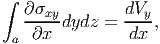
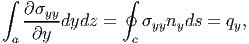
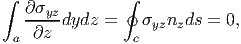
Now we are interested in the net force acting at this section, i.e.,
 | (8.2) |
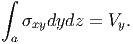
where P is called the axial force, V y and V z the shear force. Equating the components in equation (8.2) we obtain
 | (8.5) |
where the axial force and the shear force could vary along the longitudinal axis of the beam. Then, we are also interested in the net moment acting about the point (xo,y,z) due to the traction t(ex), i.e.,
![∫
M = a(yey + zez ) ∧ (σxxex + σxyey + σxzez)dydz
∫
= [(σxzy - σxyz )ex + σxxzey - σxxy]dydz.
a](main954x.png) | (8.6) |
 | (8.7) |
and the two bending moments by
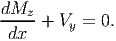
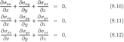
The two shear forces and bending moments are also called as the force resultants or the stress resultants in the analysis of beams. These stress resultants vary only along the longitudinal axis of the beam.Next we want to recast the static equilibrium equations in the absence of body forces, (7.6) in terms of the stress resultants. Towards this, we record the differential form of the equilibrium equations in Cartesian coordinates:
Multiply equation (8.10) with y and integrate over the cross sectional area to obtain
![∫ [ ( ) ]
∂-(yσxx)+ ∂(yσxy)-- σxy + ∂(yσxz)- dydz = 0,
a ∂x ∂y ∂z](main958x.png) | (8.13) |
Recognizing that in the first term the integration is with respect to y and z but the differentiation is with respect to another independent variable x, the order can be interchanged to obtain
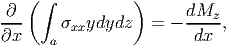 | (8.14) |
where we have used equation (8.9). To evaluate the second term in equation (8.13) we appeal to the Green’s theorem (2.275) and find that
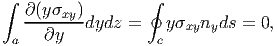 | (8.15) |
The last equality is because there are no shear stresses applied on the outer lateral surfaces of the beam. For the same reason the last term in equation (8.13) also evaluates to be zero:
 | (8.16) |
It follows from equation (8.4) that the third term in equation (8.13) is V y, i.e.,
 | (8.17) |
Substituting equations (8.14) through (8.17) in (8.13) and simplifying we obtain
 | (8.18) |
On multiplying equation (8.10) with z and integrating over the cross sectional area we obtain
![∫ [ ∂(zσxx) ∂(z σxy) ( ∂ (zσxz) )]
--------+ --------+ --------- σxz dydz = 0.
a ∂x ∂y ∂z](main964x.png) | (8.19) |
Using the equations (8.8) and (8.5) and Green’s theorem and following the same steps as above, it can be shown that equation (8.19) evaluates to requiring
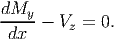 | (8.20) |
Integrating equation (8.11) over the cross sectional area we obtain
![∫ [ ]
∂σxy- ∂-σyy ∂σyz-
∂x + ∂y + ∂z dydz = 0.
a](main966x.png) | (8.21) |
Using equation (8.4), the first term in equation (8.21) evaluates to
 | (8.22) |
where by virtue of the differentiation and integration being on different independent variables, we have changed their order. Appealing to Green’s theorem (2.275), the second term in the equation (8.21) evaluates to
 | (8.23) |
where qy is the transverse loading per unit length applied on the beam. The last term in equation (8.21) evaluates as
 | (8.24) |
wherein we have again appealed to Green’s theorem (2.276) and the fact that no shear stresses are applied on the lateral surface of the beam. Substituting equations (8.22) through (8.24) in equation (8.21) it simplifies to
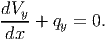 | (8.25) |
Integrating equation (8.12) over the cross sectional area we obtain
![∫ [ ]
∂σxz-+ ∂-σyz+ ∂σzz- dydz = 0.
a ∂x ∂y ∂z](main971x.png) | (8.26) |
Using the equation (8.5) and the Green’s theorem and following the procedure similar to that described above, it can be shown that equation (8.26) simplifies to
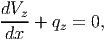 | (8.27) |
where
 | (8.28) |
Thus, we find that the three equilibrium equations reduces to four ordinary differential equations (8.18), (8.20), (8.25) and (8.27) in terms of the stress resultants in a beam.
Now, we are in a position to find the displacements and stresses in a beam subjected to some transverse loading. However, we shall initially confine ourselves to loading along the plane of symmetry of the cross section that too only along one direction.
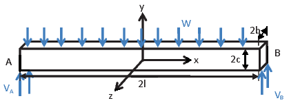
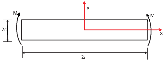
Here we assume that the beam is loaded along a single symmetric plane of the cross section. Without loss of generality we assume that this symmetric loading plane is the xy plane of the beam. For illustration, let us assume that the cross section of the beam is rectangular with depth 2c and width 2b and length 2l as shown in figure 8.2. Further, let us assume that the beam is simply supported at the ends A and B and is subjected to a uniform pressure loading W on its top surface as pictorially represented in figure 8.2. We derive the strength of materials solution before obtaining the 2 dimensional elasticity solution for this problem. While the strength of materials solution is generic, in that it is applicable for any cross section, elasticity solution is specific for rectangular cross section alone.
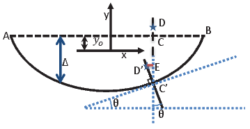
Here the displacement approach is used to obtain the solution. Hence, the main assumption here is regarding the displacement field. The assumption is that sections that are plane and perpendicular to the neutral axis (to be defined shortly) of the beam remain plane and perpendicular to the deformed neutral axis of the beam, as shown in figure 8.3. Hence, the displacement field is,
 | (8.29) |
where Δ(x) is a function of x denotes the displacement of the neutral axis of the
beam along the ey direction and yo is a constant. yo is the y coordinate of the
neutral axis before the deformation in the chosen coordinate system and is a
constant because the beam is straight. Before proceeding further let us see
why the x component of the displacement is as given. The line D′E in
figure 8.3 denotes the magnitude of the x component of the displacement.
D′E = C′D′ sin(θ) which is approximately computed as D′E = CDθ,
assuming small rotations and that there is no shortening of line segments
along the ey direction so that C′D′ = CD. Now if y coordinate of C is
yo and that of D is y, then the length of line segment CD = (y - yo).
Similarly, from the assumption that the plane sections perpendicular to
the neutral axis remain perpendicular to the deformed neutral axis, θ
=  , the slope of the tangent of the deformed neutral axis, as shown
in the figure 8.3. Therefore D′E = (y - yo)
, the slope of the tangent of the deformed neutral axis, as shown
in the figure 8.3. Therefore D′E = (y - yo) and the x component of
the displacement is -D′E since, it is in a direction opposite to the ex
direction.
and the x component of
the displacement is -D′E since, it is in a direction opposite to the ex
direction.
Now, the gradient of the displacement field for the assumed displacement (8.29) is
![( )
- [y - yo]d2Δ2 - dΔ- 0
h = ( dΔ- dx d0x 0 ) ,
dx
0 0 0](main979x.png) | (8.30) |
and therefore the linearized strain is
![( )
- [y - yo]d2Δ2 0 0
ϵ = 1-[h + ht ] = ( 0 dx 0 0) .
2
0 0 0](main980x.png) | (8.31) |
Using the one dimensional constitutive relation, σ(n) = Eϵ(n), where σ(n) and ϵ(n) are the normal stress and strain along the direction n, we obtain
![2
σ = - E [y - y ]d-Δ-,
xx o dx2](main981x.png) | (8.32) |
where we have equated the normal stress and strain along the ex direction. Substituting equation (8.32) in the equation (8.3) we obtain
![∫ 2
P = E[y - y ]d-Δ-da.
a o dx2](main982x.png) | (8.33) |
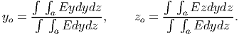
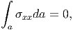
Since, in a beam there would be no net applied axial load P = 0. Solving equation (8.33) for yo under the assumption that no net axial load is applied,
 | (8.34) |
If the beam is also homogeneous then Young’s modulus, E is a constant and therefore, yo = (∫ ayda)∕(∫ ada), centroid of the cross section. Since, we have assumed that there is no net applied axial load, i.e.,
 | (8.35) |
equation (8.9) can be written as,
![∫ ∫ ∫ ∫
M = - yσ da = - y σ da + y σ da = - [y - y ]σ da,
z a xx a xx a o xx a o xx](main985x.png) | (8.36) |
where yo is a constant given in equation (8.34). Substituting equation (8.32) in equation (8.36) we obtain,
![∫ d2Δ d2Δ ∫
Mz = [y - yo]2E --2-da = ---2 [y - yo]2Eda.
a dx dx a](main986x.png) | (8.37) |
If the cross section of the beam is homogeneous, the above equation can be written as,
![2 ∫ 2
M = d-Δ-E [y - y ]2da = d--Δ EI ,
z dx2 a o dx2 zz](main987x.png) | (8.38) |
where,
![∫
2
Izz = [y - yo]da,
a](main988x.png) | (8.39) |
is the moment of inertia about the z axis.
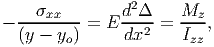
Combining equations (8.37) and (8.32) we obtain for inhomogeneous beams
![σxx d2Δ Mz
- E-(y --y-) = dx2- = ∫-[y---y-]2Eda-,
o a o](main989x.png) | (8.40) |
where yo is as given in equation (8.34). Combining equations (8.38) and (8.32) we obtain for homogeneous beams
 | (8.41) |
where yo is the y coordinate of the centroid of the cross section which can be taken as 0 without loss of generality provided the origin of the coordinate system used is located at the centroid of the cross section.
Next, we would like to define neutral axis. Neutral axis is defined as the line of intersection of the plane on which the bending stress is zero (y = yo) and the plane along which the resultant load acts.
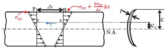
Equations (8.40) and (8.41) relate the bending stresses and displacement to the bending moment in an inhomogeneous and homogeneous beam respectively and is called as the bending equation. While these equations are sufficient to find all the stresses in a beam subjected to a constant bending moment, one further needs to relate the shear stresses to the shear force that arises when the beam is subjected to a bending moment that varies along the longitudinal axis of the beam. This we shall do next.
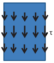
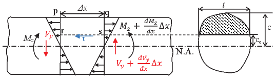
Consider a section of the beam, pqrs as shown in figure 8.4 when the beam is subjected to a bending moment that varies along the longitudinal axis of the beam. For the force equilibrium of section pqrs, the shear stress, τ, as indicated in the figure 8.4 should be
![∫ { [ ] }
τ(ΔX )t = [y - yo]-1- Mz + dMz-Δx - [y - yo]Mz-- da
a Izz dx Izz ∫
dMz ΔX
= --------- [y - yo]da,
dx Izz a](main992x.png) | (8.42) |
![∫
τ = - -Vy- [y - yo]da.
Izzt a](main993x.png) | (8.43) |
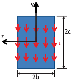
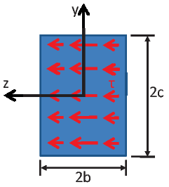
Having obtained the magnitude of this shear stress, next we discuss the direction along which this acts. For thick walled sections with say, l∕b < 20, as in the case of well proportioned rectangular beams, this shear stress is the σxy (and the complimentary σyx) component. For thin walled sections, this shear stress would act tangential to the profile of the cross section as shown in the figure 8.5b and figure 8.5c. Thus it has both the σxy and σxz shear components acting on these sections.
 (a) Thick walled rectangular
section.
(a) Thick walled rectangular
section. 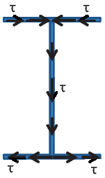 (b) Thin walled I section.
 (c) Thin walled circular section.
While the strength of material solution is generic in that it can be used for any
type of loading and cross sections of any shape as long as it is loaded in its
plane of symmetry, 2D elasticity solution has to be developed for specific
cross sections and loading scenarios. Consequently, we assume that the
cross section is rectangular in shape with width 2b and depth 2c. Thus,
the body is assumed to occupy the region in the Euclidean point space
defined by = {(x,y,z)|- l ≤ x ≤ l,-c ≤ y ≤ c,-b ≤ z ≤ b} before
the application of the load. Using the stress formulation introduced in
chapter 7, we study the response of this body subjected to three types of
load.
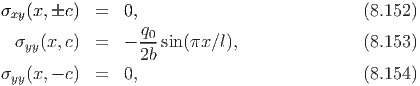
Consider the case of a straight beam subject to end moments as shown in figure 8.6. It can be seen from the figure that the top and bottom surfaces are free of traction, i.e.
 | (8.44) |
The surfaces defined by x = ±l has traction on its face such that the net force is zero but it results in a bending moment, Mz. Representing these conditions mathematically,
 | (8.45) |
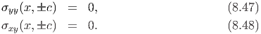
Assuming the state of stress to be plane, such that
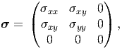 | (8.46) |
the boundary condition (8.44) translates into requiring,
For the assumed state of stress (8.46) the boundary condition (8.45) requires, Recognize that condition (8.50) holds irrespective of what the variation of the shear stress σxy is. As discussed in detail in chapter 7 (section 7.3.2), for stress formulation, we
assume that the Cartesian components of stress are obtained from a potential, ϕ
=  (x,y), called the Airy’s stress function through
 | (8.53) |
Then, we have to find the potential such that it satisfies the boundary conditions (8.47) through (8.52) and the bi-harmonic equation, Δ(Δ(ϕ)) = 0.
We express ϕ as a power series:
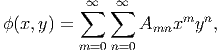 | (8.54) |
where Amn are constant coefficients to be determined from the boundary conditions and the requirement that it satisfy the bi-harmonic equation.
The choice of the stress function is based on the fact that a third order Airy’s stress function will give rise to a linear stress field, and this linear boundary loading on the ends x = ±l, will satisfy the requirements (8.49) through (8.52). Based on this observation, we choose the Airy’s stress function as
 | (8.55) |
Then, the stress field takes the form
![σxx = 6A03y + 2A12x, σyy = 6A30x + 2A21y, σxy = 2[A12y + A21x ].](main1007x.png) | (8.56) |
Substituting the above stress in boundary conditions (8.47) and (8.48) we find that A30 = A21 = A12 = 0. Thus, the Airy’s stress function reduces to,
 | (8.57) |
and the stress field becomes
 | (8.58) |
Substituting (8.60) in the boundary conditions (8.49) through (8.52), we find that (8.49) through (8.51) are satisfied identically and (8.52) requires,
 | (8.59) |
It can be verified that the Airy’s stress function (8.57) satisfies the bi-harmonic equation trivially.
Substituting (8.59) in (8.58) we obtain,
 | (8.60) |
Using the 2 dimensional Hooke’s law (7.49), the strain field corresponding to the stress field (8.60) is computed to be
Integrating (8.61) we obtain
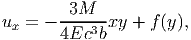 | (8.64) |
where f is an arbitrary function of y. Similarly, integrating (8.62) we obtain
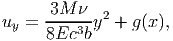 | (8.65) |
where g is an arbitrary function of x. Substituting equations (8.64) and (8.65) in equation (8.63) and simplifying we obtain
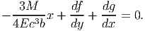 | (8.66) |
For equation (8.66) to hold,
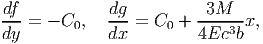 | (8.67) |
where C0 is a constant. Integrating (8.67) we obtain
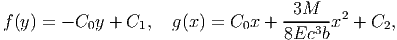 | (8.68) |
where C1 and C2 are integration constants. Substituting (8.68) in equations (8.64) and (8.65) we obtain
![3M 3M
ux = - ----3-xy - C0y + C1, uy = ----3-[x2 + νy2] + C0x + C2.
4Ec b 8Ec b](main1018x.png) | (8.69) |
The constants Ci’s are to be evaluated from displacement boundary conditions. Assuming the beam to be simply supported at the ends A and B, we require
 | (8.70) |
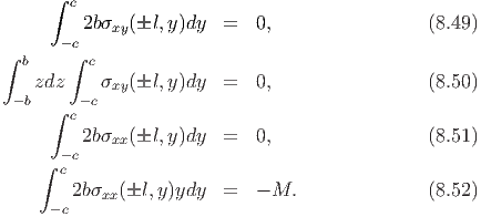
where we have assumed the left side support to be hinged (i.e., both the vertical and horizontal displacement is not possible) and the right side support to be a roller (i.e. only vertical displacement is restrained). Substituting (8.69) in (8.70) we obtain
Solving the equations (8.71) and (8.72) for C0 and C2 we obtain
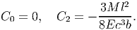 | (8.74) |
Substituting, equations (8.73) and (8.74) in the equation (8.69) we obtain the displacement field as,
![-3M--- -3M--- 2 2 2
u = - 4Ec3b xyex + 8Ec3b [x + νy - l ]ey.](main1022x.png) | (8.75) |
If the displacement boundary condition is different, then the requirement (8.70) will change and hence the displacement field.
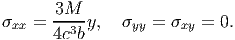
We now wish to compare this elasticity solution with that obtained by strength of materials approach. The bending equation (8.41), for rectangular cross section being studied and the constant moment case reduces to,
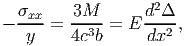 | (8.76) |
where we have used the fact that for a rectangular cross section of depth 2c and width 2b, Izz = 4c3b∕3 and that y o = 0 as the origin is at the centroid of the cross section. Using the first equality in equation (8.76) we obtain the stress field as,
 | (8.77) |
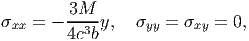
Comparing equations (8.60) and (8.77) we find that the stress field is the same in both the approaches. Then, using the last equality in equation (8.76) we obtain,
 | (8.78) |
where D1 and D2 are integration constants to be found from the displacement boundary condition (8.70). This simply supported boundary condition requires that Δ(±l) = 0, i.e.,
 | (8.81) |
Substituting (8.81) in (8.78) and the resulting equation in (8.29) we obtain
![u = - -3M---xyex + 3M--[x2 - l2]ey.
4Ec3b 8c3b](main1028x.png) | (8.82) |
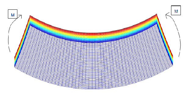
Comparing the strength of materials displacement field (8.82) with that of the elasticity solution (8.75) we find that the x component of the displacement field is the same in both the cases. However, while the y component of the displacement is in agreement with the displacement of the neutral axis, i.e., when y = 0, it is not in other cases. This is understandable, as in the strength of material solution we ignored the Poisson’s effect and used only a 1D constitutive relation. This means that the length of the filaments oriented along the y direction changes in the elasticity solution, which is explicitly assumed to be zero in the strength of materials solution. Figure 8.7 plots the deformed shape of a beam subjected to pure bending as obtained from the elasticity solution.
We shall find that this near agreement of the elasticity and strength of materials solution for pure bending of the beam does not hold for other loadings, as we shall see next.
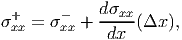
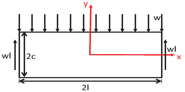
The next problem that we solve is that of a beam carrying a uniformly distributed transverse loading w along its top surface,as shown in Figure 8.8. As before the traction boundary conditions for this problem are
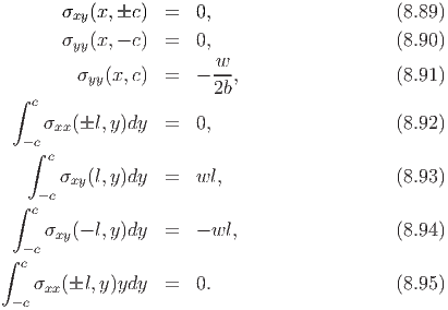
While exact point wise conditions are specified on the top and bottom surfaces, at the right and left surfaces the resultant horizontal axial force and moment are set to zero and the resultant vertical shear force is specified such that it satisfies the overall equilibrium. As before assuming plane stress conditions, (8.46), the boundary conditions (8.83) through (8.88) evaluates to, Thus, we have to chose Airy’s stress function such that conditions (8.89) through (8.95) holds along with the bi-harmonic equation.Seeking Airy’s stress function in the form of the polynomial (8.54), we try the following form,
 | (8.96) |
where Aij’s are constants. For this polynomial to satisfy the bi-harmonic equation,
 | (8.97) |
it is required that
 | (8.98) |
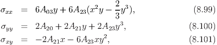
For this assumed form for the Airy’s stress function (8.96), the stress field found using equation 8.53 is,
where we have used (8.98).Substituting equation (8.101) in the boundary condition (8.89) we obtain,
 | (8.102) |
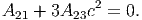
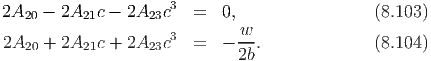
Then, using equation (8.100) in the boundary conditions (8.90),(8.91) we obtain,
Solving the above three equations for the constants A20, A21 and A23, we obtain
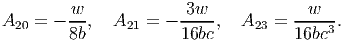 | (8.105) |
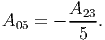
Next, substituting equation (8.99) in the boundary condition (8.92) we find that it holds for any choice of the remaining constant, A03. Similarly, when the constants, Aij are as given in (8.105), the shear stress (8.101) satisfies the boundary conditions (8.93) and (8.94). Thus, substituting equation (8.99) in the boundary condition (8.95) we obtain
![2 w [ l2 2]
A03 = - A23(l2 - -c2) = - ----- -2 - -- .
5 16bc c 5](main1042x.png) | (8.106) |
Thus, the assumed form for the Airy’s stress function (8.96) with the appropriate choice for the constants, satisfies the required boundary conditions and the bi-harmonic equation and therefore is a solution to the given boundary value problem.
Substituting the values for the constants from equations (8.105) and (8.106) in equations (8.99) through (8.101), the resulting stress field can be written as,
Having computed the stress fields, next we determine the displacement field. As usual, we use the 2 dimensional constitutive relation (7.49) to obtain the strain field as
![ϵxx = ∂ux-= σxx-- ν-σyy
∂x E{ [E ] [ ] [ ]}
w 3y 2 2 2 3y l2 2 3 y 1 y3
= 4Eb- 2c3 x - 3y - 2c- c2 - 5- + ν 1 + 2-c-- 2-c3- ,](main1044x.png) | (8.110) |
![∂u σ νσ
ϵyy = --y-= -yy-- ---xx-
∂y {E [ E ] [ ] [ ]}
-w-- 3y- 1y3- 3yν- 2 2- 2 3yν- -l2 2-
= 4Eb - 1 + 2c - 2c3 - 2c3 x - 3 y + 2c c2 - 5 ,](main1045x.png) | (8.111) |
![1 [ ∂ux ∂uy ] (1 + ν) (1 + ν) 3wx [ y2]
ϵxy = -- ----+ ---- = σxy------- = ------- ----- 1 - -2- .
2 ∂y ∂x E E 8bc c](main1046x.png) | (8.112) |
Integrating (8.110) we obtain
![w { yx [ 3 ] [ 3 y 1 y3] }
ux = ---- --- x2 - 2y2 - 3l2 + -c2 + νx 1 + ----- ----- + f(y) ,
4Eb 2c3 5 2 c 2 c3](main1047x.png) | (8.113) |
![{ [ ] [ ]
-w-- 3-y2- 1-y4- 3y2ν- 2 1-2 3y2ν- l2 2-
uy = - 4Eb y + 4 c - 8 c3 + 4c3 x - 3y - 4c c2 - 5
- g(x)},](main1048x.png) | (8.114) |
Substituting equations (8.113) and (8.114) in (8.112) and simplifying we obtain
 | (8.115) |
For equation (8.115) to hold,
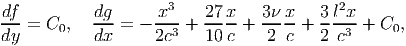 | (8.116) |
where C0 is a constant. Integrating the differential equation (8.115) we obtain
where C1 and C2 are constants to be determined from the displacement boundary condition. Assuming the beam to be simply supported at the ends A and B, we require
 | (8.120) |
where we have assumed the left side support to be hinged (i.e., both the vertical and horizontal displacement is not possible) and the right side support to be a roller (i.e. only vertical displacement is restrained). Substituting (8.114) and (8.118) in (8.120a) we obtain
Solving equations (8.121) and (8.122) for C0 and C2,
![[ ]
-l4 l2- 27- 3ν- 3l2
C0 = 0, C2 = 8c3 - 2c 10 + 2 + 2c2 .](main1054x.png) | (8.123) |
Substituting equations (8.113), (8.117) and (8.123) in (8.120b), we obtain
 | (8.124) |
Thus, the final form of the displacements is given by
![3w { yx [ 3 ] 2c3ν [ 3y 1y3 ]}
ux = ------ --- x2 - 2y2 - 3l2 + -c2 + ----x 1 - l + ---- ---- ,
8Ebc3 3 5 3 2 c 2 c3](main1056x.png) | (8.125) |
![{ [ 2 4] 3 2 [ ] 2 [ 2 ]
u = - -3w--- y + 3-y--- 1-y-- 2c- + y-ν- x2 - 1y2 - y-ν- l-- 2-
y 8Ebc3 4 c 8 c3 3 2 3 2c2 c2 5
x2c2 [27 3ν 3l2] x4 l4 l2c2 [27 3ν 3l2] }
- ----- ---+ ---+ --- + ---- ---+ ---- ---+ ---+ --- .
3 10 2 2c2 12 12 3 10 2 2c2](main1057x.png) | (8.126) |
In order to facilitate the comparison of this elasticity solution with that obtained from the strength of materials approach, we rewrite the stress and displacements field obtained using the elasticity approach in terms of the moment of inertia of the rectangular cross section of depth 2c and width 2b, Izz = 4bc3∕3, as
![{ [ ] 3 [ 3]}
ux = --w--- yx- x2 - 2y2 - 3l2 + 3-c2 + 2c-νx 1 - l + 3y-- 1y-- ,
2EIzz 3 5 3 2c 2c3](main1059x.png) | (8.130) |
![{ [ ] [ ] [ ]
--w--- 3-y2- 1-y4- 2c3 y2ν- 2 1- 2 y2ν- l2- 2-
uy = - 2EIzz y + 4 c - 8 c3 3 + 2 x - 3 y - 2c2 c2 - 5
2 2 [ 2] 4 4 2 2 [ 2] }
- x-c-- 27-+ 3ν-+ 3l- + x--- l--+ lc-- 27-+ 3ν-+ 3l- .
3 10 2 2c2 12 12 3 10 2 2c2](main1060x.png) | (8.131) |
Now, we obtain the stress and displacement field from the strength of materials approach. The bending equation (8.41) for this boundary value problem reduces to
![σxx w [ ] d2Δ
- ----= ---- l2 - x2 = E --2-,
y 2Izz dx](main1061x.png) | (8.132) |
where we have taken yo = 0 as the origin of the coordinate system coincides with the centroid of the cross section and substituted for bending moment,
![w- 2 w- [2 2]
Mz = wl(l + x) - 2 (l + x) = 2 l - x .](main1062x.png) | (8.133) |
From the first equality in equation (8.132) we obtain,
![-w-- [2 2]
σxx = - 2Izz l - x y,](main1063x.png) | (8.134) |
Using the equation (8.43) the shear stress, σxy for this cross section and loading is estimated as,
 | (8.135) |
where we have used yo = 0. Noting that V y = wl - w(l + x) = -wx, equation (8.135) simplifies to
![σ = -w--x [c2 - y2],
xy 2Izz](main1065x.png) | (8.136) |
In strength of materials solution we do not account for the variation of the σyy component of the stress. Hence,
 | (8.137) |
From solving the ordinary differential equation in the last equality in equation (8.132) we obtain,
![[ ]
--w--- 2 2 x4-
Δ = 4EIzz l x - 6 + D1x + D2 ,](main1067x.png) | (8.138) |
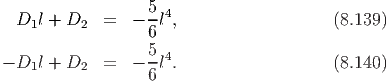
where D1 and D2 are constants to be found from the displacement boundary condition (8.120). The boundary condition (8.120a) requires that
Solving equations (8.139) and (8.140) for the constants D1 and D2 we obtain
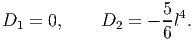 | (8.141) |
Substituting (8.141) in equation (8.138) we obtain
![w [ x4 5 ]
Δ = ------ l2x2 - ---- -l4 .
4EIzz 6 6](main1070x.png) | (8.142) |
Hence the displacement field in a simply supported beam subjected to transverse loading obtained from strength of materials approach is,
![[ ] [ ]
--w--- 2 2x3- --w--- 2 2 x4- 5-4
u = - y4EI 2l x - 3 ex + 4EI lx - 6 - 6l ey.
zz zz](main1071x.png) | (8.143) |
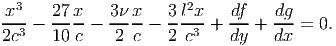
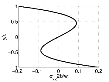
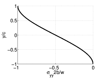
Before concluding this section let us compare the 2 dimensional elasticity solution with the strength of material solution. Comparing equations (8.136) with equation (8.129), we find that identical shear stress, σxy variation is obtained in both the approaches. However, comparing equations (8.134) and (8.127) we find that the expression for the bending stress, σxx obtained by both these approaches are different. First observe that in strength of materials solution σxx(±l,y) = 0. However, in the elasticity solution, σxx(±l,y) = wy[c2∕5 - y2∕3]∕I zz. Figure 8.9 plots the variation of σxx(±l,y)2b∕w with respect to y∕c. Moreover, at any section we find that the bending stress, σxx varies nonlinearly with respect to y in the elasticity solution. To understand how different the elasticity solution is from the strength of materials solution, in figure 8.10 we plot both the variation of the bending normal stress, σxx(0,y)2b∕w as a function of y∕c for various values of l∕c. It can be seen from the figure that for values of l∕c ≤ 1 the differences are significant but as the value of l∕c tends to get larger the differences diminishes. Also notice that the maximum bending stress max(σxx(0,y)) varies quadratically as a function of l∕c. In figure 8.11 we plot the variation of the stress σyy2b∕w with y∕c to find that its magnitude is less than 1. Thus, for typical beams with l∕c > 10, the bending stresses σxx is 100 times more than these other stresses that they can be ignored, as done in strength of materials solution.
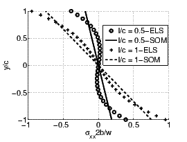 (a) For values of l∕c ≤ 1, large differences
between elasticity and strength of materials
solution.
(a) For values of l∕c ≤ 1, large differences
between elasticity and strength of materials
solution.
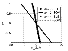 (b) For values of l∕c > 1, negligible differences
between elasticity and strength of materials
solution.
(b) For values of l∕c > 1, negligible differences
between elasticity and strength of materials
solution.
Having examined the difference in the stresses let us now examine the displacements. The maximum deflection of the neutral axis of the beam in the elasticity solution is
![5wl4 { c2 [54 6ν] }
umayx = uy(0,0) = - ------- 1 + -2 ---+ --- ,
24EIzz l 25 5](main1076x.png) | (8.144) |
obtained from equation (8.131). The corresponding value calculated from strength of materials solution (8.142) is
 | (8.145) |
Comparing equations (8.144) and (8.145) it can be seen that when l∕c ≫ 1 the results are approximately the same. Thus, again we find that for long beams with l∕c > 10 the strength of materials solution is close to the elasticity solution. Note that from equation 8.125, the x component of displacement indicates that plane sections do not remain plane. However, for well proportioned beams, i.e. beams with l∕c > 10, the deviation from being plane is insignificant.
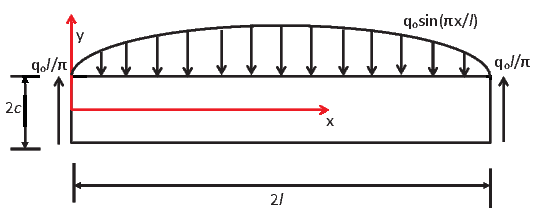
Finally, we consider a simply supported rectangular cross section beam subjected to
sinusoidally varying transverse load along its top edge as shown in Fig 8.12. Now,
we shift the coordinate origin to the left end surface of the beam. Consequently,
the beam in its initial state is assumed to occupy a region in the Euclidean point
space defined by = {(x,y,z)|0 ≤ x ≤ 2l,-c ≤ y ≤ c,-b ≤ z ≤ b}.
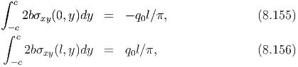
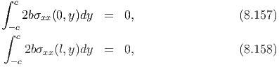
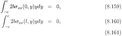
The traction boundary conditions for this problem are
The conditions (8.146) through (8.151) on assuming that the beam is subjected to a plane state of stress, translates into requiringAs before, we solve this boundary value problem using stress approach. Towards this, we assume the following form for the Airy’s stress function
![ϕ = sin(βx ){[A1 + A3 βy]sinh(βy ) + [A2 + A4 βy ]cosh(βy)} ,](main1086x.png) | (8.162) |
where Ai’s are constants to be determined from boundary conditions. It is straightforward to verify that the above choice of Airy’s stress function, (8.162) satisfies the bi-harmonic equation.
Then, the Cartesian components of the stress for the assumed Airy’s stress function (8.162) is
![2
σxx = β sin(βx ){A1 sinh (βy)+A3 [yβ sinh (βy) + 2cosh (βy )]+A2 cosh(βy)
+ A4 [βy cosh (βy) + 2sinh(βy )]},](main1087x.png) | (8.163) |
![2
σyy = - β sin (βx ){[A1 + A3 βy ]sinh (βy ) + [A2 + A4βy ]cosh(βy)} ,](main1088x.png) | (8.164) |
![2
σxy = β cos(βx ){A1 cosh(βy ) + A3 [βy cosh(βy ) + sinh(βy )] + A2 sinh (βy)
+ A4 [βy sinh(βy ) + cosh (βy )]}.](main1089x.png) | (8.165) |
Now applying the boundary condition we evaluate the constants, Ai’s. The condition 8.152 implies that
![A1 cosh(βc) + A3 [βc cosh(βc ) + sinh(βc)] + A2 sinh (βc)
+ A4 [βc sinh (βc) + cosh(βc)] = 0.](main1090x.png) | (8.166) |
![A1 cosh(βc) - A3 [βc cosh(βc ) + sinh(βc)] - A2 sinh (βc)
+ A [βc sinh (βc) + cosh(βc)] = 0.
4](main1091x.png) | (8.167) |
![A1 cosh (βc ) + A4 [βc sinh (βc) + cosh(βc)] = 0,](main1092x.png) | (8.168) |
Subtracting equations (8.166) and (8.167) we obtain,
![A2 sinh (βc) + A3 [βc cosh(βc) + sinh (βc)] = 0.](main1093x.png) | (8.169) |
We write A1 in terms of A4 using equation (8.168) as
![A1 = - A4[βc tanh(βc ) + 1].](main1094x.png) | (8.170) |
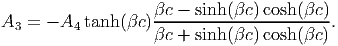
Similarly, we write A2 in terms of A3 using equation (8.169) as
![A2 = - A3 [βc coth(βc) + 1].](main1095x.png) | (8.171) |
Substituting equations (8.170) and (8.171) in (8.164)
![2
σyy = - β sin(βx ){A4 [βy cosh(βy ) - (βc tanh (βc ) + 1 )sinh (βy)]
+ A3 [βy sinh(βy ) - (βc coth(βc) + 1)cosh (βy )]}.](main1096x.png) | (8.172) |
 | (8.173) |
The boundary condition (8.153) requires
![[ ]
πx 2 βc - sinh(βc )cosh(βc)
q0sin(---) = 2β sin(βx ) ---------------------- A4.
l cosh(βc )](main1098x.png) | (8.174) |
In order for equation 8.174 to be true for all x, β = π∕l, and so A4 is determined as,
![( )
---------q0cosh--πcl-----------
A4 = π2[ πc (πc) (πc)].
4bl2 l - sinh l cosh l](main1099x.png) | (8.175) |
It can be verified that for these choice of constants, boundary conditions (8.155) through (8.160) is satisfied. Thus, we have found a stress function that satisfies the bi-harmonic equation and the traction boundary conditions and therefore is a solution to the boundary value problem.
The displacements are determined through integration of the strain displacement relations. Since the steps in its computation is same as in the above two examples, only the final results are recorded here
![u = - β-cos(βx ){A [1 + ν]sinh(βy ) + A [1 + ν ]cosh(βy)
x E 1 2
+ A3 [(1 + ν)βy sinh(βy ) + 2 cosh(βy)]
+ A4 [(1 + ν)βy cosh(βy) + 2sinh(βy )]} - C0y + C1,](main1100x.png) | (8.176) |
![β
uy = - --sin(βx ){A1[1 + ν]cosh(βy ) + A2 [1 + ν ]sinh (βy)
E
+ A3 [(1 + ν )βy cosh (βy ) - (1 - ν )sinh (βy)]
+ A [(1 + ν)βy sinh (βy) - (1 - ν)cosh(βy )]} + C x + C ,
4 0 2](main1101x.png) | (8.177) |
 | (8.178) |
The constant Ci’s determined using the above displacement conditions is
![C0 = C2 = 0, C1 = β- [A2 (1 + ν) + 2A3].
E](main1103x.png) | (8.179) |
In order to facilitate comparison of this displacement field with that obtained from strength of materials approach, the vertical displacement of the centerline is determined from equation (8.177) as
![u (x,0) = A4-β sin(βx )[2 + (1 + ν )βctanh (βc)].
y E](main1104x.png) | (8.180) |
For the case when l ≫ c, we approximately compute A4 as A4 ≈-3q0l5∕8bc3π5, and so the equation (8.180) becomes
![3q l4 (πx ) [ 1 + ν πc (πc )]
uy(x,0) = - ----0--- sin --- 1 + ---------tanh --- .
4bc3π4E l 2 l l](main1105x.png) | (8.181) |
Without going into the details, the vertical deflection of the beam computed using strength of materials approach is,
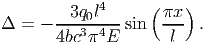 | (8.182) |
When l∕c > 10 it can be seen that both the elasticity and strength of materials solution is in agreement as expected.
 (a) Actual loading.
 (b) Load resolved along the axis of symmetry.
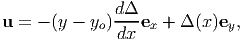
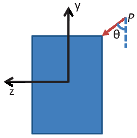
Having shown that for the symmetrical bending the strength of material approximation is robust when l∕c > 10, we proceed to use the same approximation for asymmetrical bending. In the case of asymmetrical bending the loading plane does not coincide with the plane of symmetry. As an illustration, consider the rectangular section, loaded as shown in the figure 8.13a. The applied load can be resolved along the symmetry plane, as shown in figure 8.13b. Thus, the beam bends in both the xy plane due to loading along y direction and the xz plane due to loading along the z direction. As per the strength of materials assumption that the plane section before deformation remain plane and that the sections normal to the neutral axis, remain normal after the deformation, the displacement field for this case is,
![{ }
u = - [y - y]dΔy- + [z - z ]dΔz- e + Δ (x)e + Δ (x)e ,
o dx o dx x y y z z](main1109x.png) | (8.183) |
where Δy(x) and Δz(x) are yet to be determined functions of x, yo and zo are constants. The above displacement field is obtained by superposing the bending displacement due to transverse loading along one symmetric plane, say xy plane, (8.29) and the displacement filed due to loading along another symmetric plane say xz (obtained by substituting z in place of y in equation (8.29)). Recollect from section 7.5.2 that for the linear elastic material that we are studying, we can superpose solutions as long as the displacements are small.
As required in the displacement approach, we next compute the linearized strain corresponding to the displacement field, (8.183) as
![( { 2 2 } )
- [y - yo]ddΔxy2 + [z - zo]ddΔxz2- 0 0
ϵ = |( 0 0 0|) .
0 0 0](main1110x.png) | (8.184) |
Then, using the 1 dimensional constitutive relation, the stress is obtained as
![{ }
d2Δy d2Δz
σxx = - E [y - yo]---2- + [z - zo]---2 .
dx dx](main1111x.png) | (8.185) |
Substituting (8.185) in equation (8.3) and using the condition that no axial load is applied we obtain
![{ }
∫ ∫ d2Δy d2Δz
E [y - yo]---2-+ [z - zo]---2- dydz = 0.
a dx dx](main1112x.png) | (8.186) |
For equation (8.186) to hold we require that
![∫ ∫ ∫ ∫
E [y - yo]dydz = 0, E [z - zo]dydz = 0,
a a](main1113x.png) | (8.187) |
since in equation (8.186) Δy and Δz are independent functions of x and in particular Δy ≠ -kΔz, where k is a constant. From equation (8.187) we obtain,
 | (8.188) |
If the beam is also homogeneous then Young’s modulus, E is a constant and therefore,
 | (8.189) |
the y and z coordinates of the centroid of the cross section. Without loss of generality the origin of the coordinate system can be assumed to be located at the centroid of the cross section and hence yo = zo = 0.
Since, we have assumed that there is no net applied axial load, i.e.,
 | (8.190) |
equation (8.9) and (8.8) can be written as,
where yo and zo are constants as given in equation (8.188). Substituting equation (8.185) in equation (8.191) we obtain,![∫ ∫ ∫ ∫
2 d2Δy d2 Δz
Mz = [y - yo]E -dx2-dydz + [y - yo][z - zo]E -dx2- dydz
a a
d2Δ ∫ ∫ d2Δ ∫ ∫
= ----y [y - yo]2Edydz + ----z [y - yo][z - zo]Edydz.
dx2 dx2
a a](main1118x.png) | (8.193) |
![d2Δ ∫ ∫ d2Δ ∫ ∫
Mz = ---2yE [y - yo]2dydz + ----z2 E [y - yo][z - zo]dydz
dx dx
a a 2 2
= d-Δy-EI + d-Δz-EI ,
dx2 zz dx2 yz](main1119x.png) | (8.194) |
![∫ ∫ ∫ ∫
Izz = [y - yo]2dydz, Iyz = [y - yo][z - zo]dydz,
a a](main1120x.png) | (8.195) |
are the moment of inertia about the z axis, the axis about which the applied forces produces a moment, Mz and the product moment of inertia. Substituting equation (8.185) in equation (8.192) we obtain,
![∫ ∫ ∫ ∫
d2Δy- 2 d2Δz-
My = - [y - yo][z - zo]E dx2 dydz - [z - zo] E dx2 dydz
a a
d2Δ ∫ ∫ d2Δ ∫ ∫
= - ---2y [y - yo][z - zo]Edydz - ----z2 [z - zo]2Edydz.
dx dx
a a](main1121x.png) | (8.196) |
![d2Δy ∫ ∫ d2 Δz ∫ ∫
My = - ---2-E [y - yo][z - zo]dydz - ----2 E [z - zo]2dydz
dx a dx a
2 2
= - d-Δy-EI - d-Δz-EI ,
dx2 yz dx2 yy](main1122x.png) | (8.197) |
![∫ ∫
I = [z - z ]2dydz,
yy o
a](main1123x.png) | (8.198) |
is the moment of inertia about the y axis, the axis about which the applied forces produces a moment, My. Solving equations (8.194) and (8.197) for Δy and Δz we obtain,
![d2Δy- IyzMy--+-IyyMz-- d2Δz- IyzMz-+-IzzMy--
dx2 = E [IyyIzz - I2yz], dx2 = - E [IyyIzz - I2yz].](main1124x.png) | (8.199) |
Substituting (8.199) in (8.185) we obtain
![IyzMy--+-IyyMz- IyzMz--+-IzzMy-
σxx = - [y - yo] I I - I2 + [z - zo] I I - I2 ,
yy zz yz yy zz yz](main1125x.png) | (8.200) |
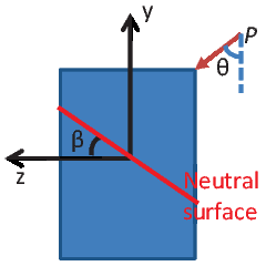
where yo and zo are as given in equation (8.189). Equation (8.200) gives the bending normal stress when a cross section is subjected to both My and Mz bending moments or when the cross section is subjected to a bending moment about an axis for which the product moment of inertia is not 0, i.e., loading is not along a plane of symmetry.
Before proceeding further, a few observations on equation (8.200) have to be made. It is clear from the equation (8.200) that the bending normal stress varies linearly over the cross sectional surface. As in the case of symmetrical bending, there exist a surface which has zero bending normal stress. This zero bending normal stress surface, called as the neutral surface is defined by
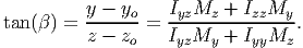 | (8.201) |
Figure 8.14 shows a typical neutral surface for a beam with rectangular cross section subjected to transverse loading not in the plane of symmetry of the cross section.
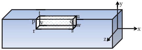
Having found the bending normal stress, next we find the bending shear stress. Towards this, we consider the equilibrium of a cuboid pqrstuvw as shown in figure 8.15, taken from a beam subjected to asymmetric bending moment that varies along the longitudinal axis of the beam. Note that on this cuboid, bending normal stress σxx- acts on the face prtv and σ xx+ acts on the face qsuw, shear stress, σxy acts in plane rsvw and shear stress, σxz acts in plane tuvw. Now, the force balance along the x direction requires that
![∫ ∫
σxy(Δx )(b - z ) + σxz(Δx )(c - y) + [σ+xx - σ-xx]dzdy = 0,
a](main1129x.png) | (8.202) |
where we have assumed that constant shear stresses act on faces rsvw and pqrs and that the bending normal stress varies linearly over the faces prtv and qsuw as indicated in equation (8.200). Appealing to Taylor’s series, we write,
 | (8.203) |
truncating the series after first order term, since our interest is in the limit (Δx) tending to zero. Differentiating (8.200) with respect to x we obtain,
![[ ]
dσxx [y - yo] dMz dMy
-----= - ----------2-- Iyy-----+ Iyz-----
dx [IzzIyy - Iyz] dx dx [ ]
--[z---zo]--- dMz-- dMy--
+ [I I - I2 ] Iyz dx + Izz dx
zz yy yz](main1131x.png) | (8.204) |
![dσ [y - y ] [z - z ]
--xx-= - ---------o---[- IyyVy + IyzVz] + --------o----[- IyzVy + IzzVz].
dx [IzzIyy - I2yz] [IzzIyy - I2yz]](main1132x.png) | (8.205) |
Substituting equation (8.205) in (8.203) and using the resulting equation in (8.202) we obtain
![∫c( ∫b )
[IyyVy - IyzVz ] { }
σxy(b - z) + σxz(c - y) = --[I-I-----I2-]- ( [y - yo] dz) dy
zz yy yz y z
b( c )
[IzzVz - IyzVy]∫ { ∫ }
- -----------2-- [z - zo] dy dz,
[IzzIyy - Iyz] z ( y )](main1133x.png) | (8.206) |
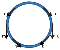
On the other hand since the direction of the shear stress is well defined in thin walled sections. It is going to be tangential to the cross section at the point of interest, as in the case of symmetric bending. Further, by virtue of the section being thin walled, we assume the shear stresses to be uniform across its thickness, t. Now, the shear stress, τ acting as shown in figure 8.16 balances the imbalance created due to the variation of the bending normal stresses along the longitudinal axis of the beam. Following the same steps as in the case of thick walled cross sections detailed above, it can be shown that
![{ ∫ ∫ }
1 [IyyVy - IyzVz] [IzzVz - IyzVy]
τ = - -- -----------2--- [y - yo]dydz + -----------2-- [z - zo]dydz ,
t [IzzIyy - Iyz] a [IzzIyy - Iyz] a](main1134x.png) | (8.207) |
where the area over which the integration is to be performed is the shaded region
shown in figure 8.16. If one is to use polar coordinates to describe the cross section
and defining ro =  and β = tan -1(y
o∕zo), the equation (8.207) can be
written as,
and β = tan -1(y
o∕zo), the equation (8.207) can be
written as,
![[IyyVy - IyzVz] ∫ α [ ro ]
τ = - -----------2--- r2 sin (θ) - --sin(β) d θ
[IzzIyy - Iyz] ϕ r ∫
[IzzVz --IyzVy-] α 2[ ro ]
- [I I - I2 ] r cos(θ) - r cos(β ) dθ,
zz yy yz ϕ](main1136x.png) | (8.208) |
While this representation is convenient in cases where the section is not made up of straight line segments, a representation using the perimeter length, s, of the cross section is useful when the section is made up of straight line segments. Thus, the expression for the shear stress in terms of the perimeter length as shown in figure 8.16 is,
![[IyyVy - IyzVz ]∫ s [IzzVz - IyzVy]∫ s
τ = - -----------2--- [rsin (θ)- yo]ds - -----------2-- [r cos(θ)- zo]ds,
[IzzIyy - Iyz] 0 [IzzIyy - Iyz] 0](main1137x.png) | (8.209) |
where now r and θ have to be expressed as a function of s. Here we have used the relation, ds = rdθ to obtain (8.209) from (8.208).
Thus, integrating the ordinary differential equations (8.199) we obtain the deflections of the beam along the y and z directions and hence the displacement field for the beam, (8.183) can be computed. Using equation (8.200) the bending normal stress is evaluated. While these calculations are the same for thin or thick walled sections, the shear stress estimation is different. We could not find the shear stresses in case of thick walled sections using the strength of materials approach. However, equation (8.207) gives the shear stresses in thin walled sections. This completes the solution to asymmetrical bending problem.
Having found the solution to symmetrical and asymmetrical bending, in this section we find where the load has to be applied so that it produces no torsion.
Shear center is defined as the point about which the external load has to be applied so that it produces no twisting moment.
Recall from equation (8.7) the torsional moment due to the shear force σxy and σxz about the origin is,
![∫
Mx = [σxzy - σxyz]dydz.
a](main1139x.png) | (8.210) |
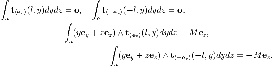
Since, ∫ aσxzdydz = V z and ∫ aσxydydz = V y, the moment about some other point (ysc,zsc) would be,
![∫
M sc= [σxzy - σxyz]dydz - Vzysc + Vyzsc.
x a](main1140x.png) | (8.211) |
If this point (ysc,zsc) is the shear center, then Mxsc = 0. Thus, we have to find y sc and zsc such that,
![∫
[σ y - σ z]dydz - V y + V z = 0,
a xz xy z sc y sc](main1141x.png) | (8.212) |
holds. We have two unknowns but only one equation. Hence, we cannot find ysc and zsc uniquely, in general. If the loading is such that only shear force V y is present, then
![∫
-1-
zsc = V [σxyz - σxzy ]dydz.
y a](main1142x.png) | (8.213) |
Similarly, if V y = 0,
![1 ∫
ysc = --- [σxzy - σxyz ]dydz.
Vz a](main1143x.png) | (8.214) |
Equations (8.213) and (8.214) are used to find the coordinates of the shear center with respect to the chosen origin of the coordinate system, which for homogeneous sections is usually taken as the centroid of the cross section. Thus, the point that (ysc,zsc) are the coordinates of the shear center from the origin of the chosen coordinate system which in many cases would be the centroid of the section cannot be overemphasized. In the case of thin walled sections which develop shear stresses tangential to the cross section, σxy = -τ sin(θ) and σxz = τ cos(θ), where τ is the magnitude of the shear stress and θ is the angle the tangent to the cross section makes with the z direction.
By virtue of the shear stress depending linearly on the shear force (see equations (8.43) and (8.207)), it can be seen that the coordinates of the shear center is a geometric property of the section.
Next, to illustrate the use of equations (8.213) and (8.214) we find the shear center for some shapes.
The first section that we consider is a thick walled rectangular section as shown in figure 8.17 having a depth 2c and width 2b. The chosen coordinate basis coincides with the two axis of symmetry that this section has and the origin is at the centroid of the cross section.
First, we shall compute the z coordinate of the shear center zsc. For this only shear force V y should act on the cross section. Shear force V y would be caused due to loading along the xy plane, a plane of symmetry for the cross section. Therefore the shear stress, σxy is computed using (8.43) as
![∫ c [ 2]
σxy = - ------Vy------(2b) ydy = 3Vy- 1 - y-- ,
2b(2b(2c)3∕12 ) y 8bc c2](main1146x.png) | (8.215) |
where we have used the fact that yo = 0, since the origin is located at the centroid of the cross section. Further, for this loading σxz = 0. Substituting (8.215) and σxz = 0 in (8.213) we obtain
![∫ b ∫ c[ 2]
zsc = -3-- zdz 1 - y--dy = 0.
8bc -b -c c2](main1147x.png) | (8.216) |
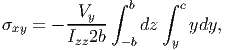
Next, we shall compute the y coordinate of the shear center ysc. Now, only shear force V z should act. This shear force would be produced by loading along the xz plane, also a plane of symmetry for the cross section. This loading produces a shear stress as shown in figure 8.17b whose magnitude is again computed using (8.43) as
![∫ [ ]
Vz b 3Vz z2
σxz = - ---------3----(2c) zdz = ---- 1 - -2- .
2c(2c(2b) ∕12) z 8bc b](main1148x.png) | (8.217) |
and σxy = 0. Substituting (8.217) in (8.214) we obtain
![∫ c ∫ b[ 2]
ysc = -3-- ydy 1 - z--dz = 0.
8bc - c -b c2](main1149x.png) | (8.218) |
Thus, for the rectangular cross section, the shear center is located at the origin of the coordinate system, which in turn is the centroid of the cross section. Hence, the shear center coincides with the centroid of the cross section.
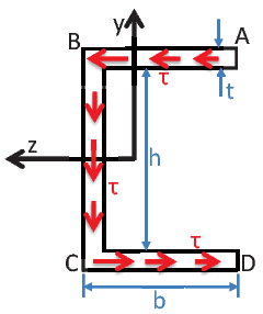
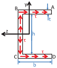
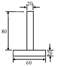
The next section that we study is the channel section with orientation and dimensions as shown in figure 8.18. The flange and web thickness of the channel is the same. Before proceeding to compute the shear center the other geometric properties, the centroid and the moment of inertia’s for the cross section is computed. The origin of the coordinate system being used is at the centroid of the cross section. Then, the distance from the centroid of the cross section to the top most fiber of the cross section AB is yAB = c = h∕2 + t. Similarly, the distance of the left most fiber in the web of the cross section, BC is zBC = (ht + 2b2)∕(2(h + 2b)). Now,
![Iyz = 0, (8.219)
1 [ ] 1
Izz = --- th3 + 2bt3 + -bt(h + t)2, (8.220)
12 2](main1152x.png)
![[ ] ( )2 ( )2
Iyy = 1-- ht3 + 2tb3 + ht zBC - t- + 2bt b- zBC
12 2 2
1 [ ] ht( b(b - 2t))2 bt ( h(b - t) )2
= --- ht3 + 2tb3 + --- --------- + -- -------- .
12 4 (h + 2b) 2 (h + 2b )](main1153x.png) | (8.221) |
Towards computing the location of the shear center along the z direction, we first compute the shear stress acting on the cross section due to a shear force V y alone. The magnitude of the shear stress, τ is found using (8.209) as
![(
| - Vy-(h+t)∫ sds 0 ≤ s ≤ (b - -t)
||| IVzyz[2(h+t)0∫b-t∕2 2
|||| - Izz --2-- 0 ds
{ ∫s [ (h+t)- ( t)] ] ( t) ( -t)
τ = + [b- t∕2 2 - s - b + 2 ds b - 2 ≤ s ≤ b + h + 2 .
|||| Vy- (h+t)∫b-t∕2 (h+t)∫s
||| - Izz∫ 2 0[ ds -( 2 b+h+)t]∕2ds] ( )
|( + b+h+t∕2 (h+t)- s - b + t ds b + h + t ≤ s ≤ (2b + h)
b- t∕2 2 2 2](main1154x.png) | (8.222) |
Evaluating the integrals and simplification yields,
![( )
(| - -Vy-(h + t)s 0 ≤ s ≤ b - t
||{ 2IVzzy [ ( t) ( t)2 2
τ = - 2Izz- (h + t) b - 2 - s2 + b - 2 .
|| + (h + 2b)(s - b + t)] (b - t) ≤ s ≤ (b + h + t)
|( -Vy- 2 ( 2 t) 2
2Izz(h + t)(2b + h - s) b + h + 2 ≤ s ≤ (2b + h)](main1155x.png) | (8.223) |
Since this shear stress has to be tangential to the cross section, it would be σxz component in the flanges and σxy component in the web. Rewriting equation (8.213) in terms of integration over the perimeter length,
![t ∫ So
zsc = --- [σxyr cos(θ) - σxzr sin (θ)]ds,
Vy 0](main1156x.png) | (8.224) |
where So is the total length of the perimeter of the cross section. Evaluating the above equation, (8.224) for the channel section yields,
![{
t ∫ b-t∕2 (h + t)
zsc = ---- (h + t)s-------ds
2Izz 0 2
∫ 2b+h
+ (h + t)(2b + h - s)(h-+-t)ds
b+h+t∕2 2
( ) ∫ b+h+t∕2 [ ( ) ( )2
- z - t- (h + t) b - t- - s2 + b - t-
BC 2 b-t∕2 2 2
( ) ] }
+ (h + 2b) s - b + t- ds .
2](main1157x.png) | (8.225) |
![2 2 [ ] 2
zsc = t(h-+-t)-(2b --t)-+ zBC - t- (h + 6b - 2t)t(h +-t)-.
16Izz 2 12Izz](main1158x.png) | (8.226) |
For computing the location of the shear center along the y direction, we next compute the shear stress acting on the cross section due to a shear force V z alone. The magnitude of the shear stress, τ is found using (8.209) as
![( ∫ ( )
|| - IVz 0s(s + zBC - b)ds 0 ≤ s ≤ b - t2
||| yVyz[∫ b-t∕2
||| - Iyy 0 (s + zBC - b])ds
|||{ ( t)∫ s ( t) ( t)
+ [zBC - 2 b-t∕2ds b - 2 ≤ s ≤ b + h + 2
τ = | - -Vz ∫ b-t∕2(s + z - b)ds .
|||| Iyy( 0 )∫ BC
||| + zBC - t2 bb+-ht+∕t2∕2ds
||| ∫s ] ( t)
( + b+h+t∕2(h - s + zBC + b)ds b + h + 2 ≤ s ≤ (2b + h)](main1159x.png) | (8.227) |
Integrating the above equation we obtain,
![( [ 2 ] ( )
|| - VIyzy- s2-+ (zBC - b)s 0 ≤ s ≤ b - t2
|||| V [(2b-t)2 (2b-t)
||| - Iyzy- --8---+ (zBC - b)--2--
||| ( t)( (2b-t))] ( t) ( t)
{ + z[BC - 2 s - 2 b - 2 ≤ s ≤ b + h + 2
τ = | - Vz- (2b-t)2-+ (z - b)(2b-t) .
||| Iyy( 8 ) BC 22
|||| + zBC - t2 (h + t) - s2-
||| + (b+h+t∕2)2
|( 2 ( t)] ( t)
+ (zBC + b + h) s - b - h - 2 b + h + 2 ≤ s ≤ (2b + h )](main1160x.png) | (8.228) |
Since this shear stress has to be tangential to the cross section, as before, it would be σxz component in the flanges and σxy component in the web. Rewriting equation (8.214) in terms of integration over the perimeter length,
![∫ So
ysc = - -t- [σxyr cos(θ ) - σxzr sin (θ )]ds,
Vz 0](main1161x.png) | (8.229) |
where So is the total length of the perimeter of the cross section. Evaluating the above equation, (8.229) for the channel section yields,
![{ ∫ b-t∕2[ 2 ]
y = - -t- (h-+-t) s- + (z - b)s ds
sc Iyy 2 0 2 BC
( ) ∫ b+h+t∕2[
t- (2b---t)2 (2b --t)
- zBC - 2 b-t∕2 8 + (zBC - b) 2
( ) ( ) ]
+ z - -t s - (2b---t)- ds
BC 2 2
∫ 2b+h [ 2 ( ) 2
- (h-+-t) (2b---t)-+ (zBC - b)(2b --t)-+ zBC - t- (h + t) - s-
2 b+h+t∕2 8 2 2 2
(b + h + t∕2)2 ( t )] }
+ --------------+ (zBC + b + h) s - b - h - -- ds
2 2](main1162x.png) | (8.230) |
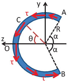
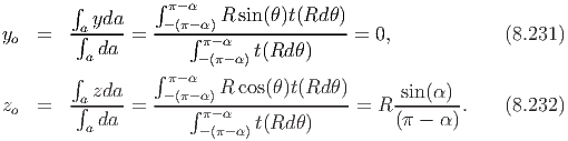
The final section that we use to illustrate the procedure to find the shear center is an arc of a circular section with radius R and a uniform thickness t. The arc is assumed to span from -(π - α) ≤ θ ≤ (π - α). Thus, it is symmetrical about the z direction. For convenience, we assume the origin of the coordinate system to be located at the center of the circle. First, we compute the centroid of the cross section,
Here we have identified yo and zo with the coordinates of the centroid of the cross section, since it is homogeneous. Next, we compute the moment of inertias about the centroid,![∫ ∫
2 π- α 2
Izz = [y - yo] da = [R sin(θ) - 0 ]t(Rd θ)
a - (π- α) [ ]
= R3t π - α + 1-sin(2α ) ,
2](main1166x.png) | (8.233) |
![∫ ∫ π- α
Iyz = a[y - yo][z - zo]da = - (π- α)[R sin(θ) - 0 ][R cos(θ) - zo]t(Rd θ) = 0.](main1167x.png) | (8.234) |
![∫ ∫ π- α
Iyy = [z - zo]2da = [R cos(θ) - zo]2t(Rd θ)
a - (π- α)
[ ( z2) 1 zo ]
= R3t 1 + 2 -o2- (π - α ) - --sin(2α ) - 4--sin(α)
R [2 R ]
3 sin2(α ) 1
= R t π - α - 2 π----α-- 2-sin(2α ) ,](main1168x.png) | (8.235) |
Towards computing the z coordinate of the shear center, we compute the shear stress distribution in the circular arc when only shear force V y is acting on the cross section. The magnitude of the shear stress, τ is found using (8.208) as,
![Vy ∫ π-α 2 Vy 2
τ = - --- R sin(θ)dθ = - --R [cos(α) + cos(ϕ)].
Izz ϕ Izz](main1169x.png) | (8.236) |
This shear stress would act tangential to the cross section at every location as indicated in figure 8.19a. Therefore, σxy = -τ cos(ϕ) and σxz = τ sin(ϕ), where ϕ is the angle the tangent makes with the y axis. Appealing to equation (8.213) we obtain,
![1 ∫ π-α
zsc = ---- [τ cos(ϕ)(R cos(ϕ)) + τ sin(ϕ)(R sin(ϕ))]tRd ϕ
Vy -(π- α)
R4t ∫ π-α 4[(π - α) cos(α ) + sin(α )]
= ---- [cos(α) + cos(ϕ)]dϕ = R -------------------------,
Izz -(π- α) [2 (π - α) + sin(2α )]](main1170x.png) | (8.237) |
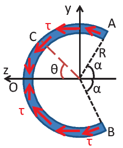
Next, for computing the y coordinate of the shear center, we compute the shear stress distribution in the circular arc when only shear force V z is acting on the cross section. The magnitude of the shear stress, τ is found using (8.208) as,
![∫ π-α [ ]
τ = - Vz- R2 cos(θ) - sin(α)-- dθ
Iyy ϕ (π - α)
V [ ϕ ]
= - --z R2 sin(α )--------- sin(ϕ) .
Iyy (π - α)](main1171x.png) | (8.238) |
![1 ∫ π-α
ysc = --- [τ cos(ϕ)(R cos(ϕ)) + τ sin(ϕ )(R sin(ϕ))]tRd ϕ
Vz -(π-α)
R4t ∫ π- α [ ϕ ]
= - ---- sin(α )--------- sin(ϕ) dϕ = 0,
Iyy - (π-α) (π - α)](main1172x.png) | (8.239) |
By virtue of the zsc being greater than R, the shear center is located outside the cross section. Hence, for the loading to pass through the shear center similar issues as discussed in the channel section exist.
In this chapter we solved boundary value problems corresponding to bending of straight, prismatic members. We obtained the solution - the stress and displacement field - by assuming the displacement field in the strength of materials approach and the stress field in the elasticity approach. We also compared the solutions and found good agreement between the solution obtained by both these approaches, when the length to depth ratio of these members are greater than 10, for the case when the loading passes through a plane of symmetry. Then, we studied asymmetric bending and obtained the solution by starting with an assumption on the displacement field. Though we did not obtain the elasticity solution for this case, it can be obtained by using principle of superposition and leave it as an exercise to the student to work the details. Then we introduced an concept called the shear center. It is the point about which the external load has to be applied so that there is no twisting of cross section. We outlined a method to find this shear center and illustrated the same for three sections.

![∂u 3M
ϵxx = ---x = - ------y, (8.61)
∂x 4Ec3b
ϵ = ∂uy- = ν -3M---y, (8.62)
yy ∂y 4Ec3b
1 [ ∂u ∂u ]
ϵxy = -- --x-+ ---y = 0. (8.63)
2 ∂y ∂x](main1012x.png)
![[ ] [ ]
3w-- l2 2- -3w- 2 2- 3
σxx = - 8bc c2 - 5 y + 8bc3 x y - 3y , (8.107)
[ 3 ]
σ = - w-- 1 + 3y-- 1y-- , (8.108)
yy 4b 2c 2c3
[ 2]
σxy = 3wx-- 1 - y-- . (8.109)
8bc c2](main1043x.png)
![f(y) = C0y[ + C1, ] (8.117)
x2- 27- 3ν- 3l2 -x4
g(x) = 2c 10 + 2 + 2c2 - 8c3 + C0x + C2, (8.118)
(8.119)](main1051x.png)
![[ ]
l4 l2 27 3ν 3l2
C0l + C2 = ---3 - --- ---+ ---+ --2 , (8.121)
8c 2c[ 10 2 2c ]
-l4 l2- 27- 3ν- 3l2
- C0l + C2 = 8c3 - 2c 10 + 2 + 2c2 . (8.122)](main1053x.png)
![w [ 2c2 2y2]
σxx = ---- x2 - l2 +--- - ---- y, (8.127)
2Izz ( 5 ) 3
-w-- y3- 2 2-3
σyy = 2I 3 - cy - 3c , (8.128)
wzz ( )
σxy = ----x c2 - y2 . (8.129)
2Izz](main1058x.png)
![∫ ∫ ∫ ∫
M = - yσ da = - yσ da + y σ da = - [y - y ]σ da,
z a xx a xx a o xx a o xx
(8.191)
∫ ∫ ∫ ∫
M = zσ da = zσ da - z σ da = [z - z ]σ da, (8.192)
y a xx a xx a o xx a o xx](main1117x.png)