10 Bending of Curved Beams

Chapter 10
Bending of Curved Beams

10.1 Overview

Till now, we have been studying members that are initially straight. In this chapter, we shall study the bending of beams which are initially curved. We do this by restricting ourselves to the case where the bending takes place in the plane of curvature. This happens when the cross section of the beam is symmetrical about the plane of its curvature and the bending moment acts in this plane. As we did for straight beams, we first obtain the solution assuming sections that are initially plane remain plane after bending. The resulting relation between the stress, moment and the deflection is called as Winkler-Bach formula. Then, using the two dimensional elasticity formulation, we obtain the stress and displacement field without assuming plane sections remain plane albeit for a particular cross section of a curved beam subjected to a pure bending moment or end load. We conclude by comparing both the solutions to find that they are in excellent agreement when the beam is shallow.

Before proceeding further, we would like to clarify what we mean by a curved beam. Beam whose axis is not straight and is curved in the elevation is said to be a curved beam. If the applied loads are along the y direction and the span of the beam is along the x direction, the axis of the beam should have a curvature in the xy plane. On the hand, if the member is curved on the xz plane with the loading still along the y direction, then it is not a curved beam, as this loading will cause a bending as well as twisting of the section. Thus, a curved beam does not have a curvature in the plan. Arches are examples of curved beams.

10.2 Winkler-Bach formula for curved beams

(a) Elevation view: projection in the xy plane. (b) Isotropic view.

Figure 10.1: Schematic of bending of a curved beam

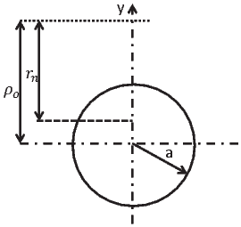
As mentioned before, in this section we obtain the stress field assuming, sections that are plane before bending remain plane after bending. Consequently, a transverse section rotates about an axis called the neutral axis as shown in figure 10.1. Let us examine an infinitesimal portion of a curved beam enclosing an angle Δϕ. Due to an applied pure bending moment M, the section AB rotates through an angle δ(Δϕ) about the neutral axis and occupy the position A′B′. SN denotes the surface on which the stress is zero and is called the neutral surface. Since, the stress is zero in this neutral surface, the length of the material fibers on this plane and oriented along the axis of the beam would not have changed. However, fibers above the neutral surface and oriented along the axis of the beam would be in compression and those below the neutral surface and oriented along the axis of the beam would be in tension. Hence, for a fiber at a distance y from the neutral surface, its length before the deformation would be (r_n - y)Δϕ, where r_n is the radius of curvature of the neutral surface. The change in length of the same fiber after deformation due to the applied bending moment, M would be -y(δ(Δϕ)). Note that the negative sign is to indicate that the length reduces when y is positive for the direction of the moment indicated in the figure 10.1. Thus, the linearized strain is given by,

y(δ(Δ ϕ)) ϵ = - -------------. (rn - y)(Δ ϕ)

(10.1)

It is assumed that the lateral dimensions of the beam are unaltered due to bending, i.e. the Poisson’s effect is ignored. Hence, the quantity y remains unaltered due to the deformation. Now, to estimate the quantity δ(Δϕ)∕(Δϕ), we observe from figure 10.1a that

SN = r(Δ ϕ + δ(Δ ϕ)),

(10.2)

where r is the radius of curvature of the neutral axis after bending. However, by virtue of it being neutral surface, its length is unaltered and therefore

SN = rnΔ ϕ.

(10.3)

Equating equations (10.2) and (10.3) and simplifying we obtain

δ(Δ ϕ) rn -------= ---- 1. Δ ϕ r

(10.4)

Substituting equation (10.4) in (10.1) we obtain,

y [ rn ] ϵ = - r----y- r--- 1 . n

(10.5)

Having obtained the strain, the expression for the stress becomes

--y---[ rn- ] σ = - E r - y r - 1 , n

(10.6)

where E is the Young’s modulus and we have appealed to one dimensional Hooke’s law to relate the strain and the stress.

Since, we assume that the section is subjected to pure bending moment and in particular no axial load, we require that

∫ ∫ y [rn ] σda = - E ------- ---- 1 da = 0, a a rn - y r

(10.7)

where we have used (10.6). Since, r_n and r are constants for a given section and r ≠ r_n, when the beam deforms, for equation (10.7) to hold,

∫ Ey ------da = 0. a rn - y

(10.8)

We have to find r_n such that (10.8) holds. Observing that y∕(r_n - y) = r_n∕(r_n - y) - 1, equation (10.8) can be simplified as

∫ ∫ rn --E---da - Eda = 0. arn - y a

(10.9)

If the section is homogeneous, Young’s modulus is constant over the section and therefore the above equation can be written as,

A rn = ∫---da- a rn-y

(10.10)

Assuming the bending moment at the section being studied is M, as shown in section 8.1, equation (8.9),

∫ M = - yσda, a

(10.11)

where we have assumed that the origin of the coordinate system is located at the neutral axis of the section; consistent with the assumption made while obtaining the expression for the strain. Substituting equation (10.7) in (10.11) and rewriting we obtain,

[r ]∫ y2 [ r ]∫ [ y ]
M = --n- 1 E ------da = -n-- 1 E rn -------- y da
r a rn - y r [a ∫ rn - y ∫ ]
[ rn ] y
= ---- 1 rn E ------da - Eyda .
r a rn - y a

(10.12)

It follows from (10.8) that the first integral in the above equation is zero. Thus, equation (10.12) simplifies to

[rn ] M ---- 1 = - ∫------. r aEyda

(10.13)

Then, combining equation (10.6) and (10.13) we obtain

[rn ] M σ rn - y - ---- 1 = ∫-------= --------, r aEyda E y

(10.14)

where r_n is obtained by solving (10.9). If the section is homogeneous that is E is constant over the section equation (10.14) simplifies to,

[ ] - E rn-- 1 = ∫-M--- = σ rn --y, r ayda y

(10.15)

where r_n is obtained by solving (10.10). Note that in these equations y is measured from the neutral axis of the section and the bending moment that increases the curvature (decreases the radius of curvature) is assumed to be positive.

Thus, given the moment in the section, using equation (10.14) or (10.15), we can estimate the stress (σ) distribution in the section and/or the deformed curvature (r) of the beam. These equations are called Winkler-Bach formula for curved beams.

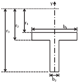
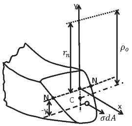
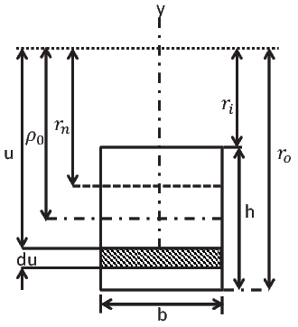
Figure 10.2: Parameters for a rectangular section to compute r_n

Next, we illustrate a technique to find the radius of curvature of the neutral surface, r_n for a homogeneous rectangular section. Consider a rectangular section shown in figure 10.2 where ρ_o denotes the radius of curvature of the centroid of the cross section, r_i the radius of curvature of the topmost fiber of the cross section and r_o the radius of curvature of the bottommost fiber of the cross section. Let u = r_n - y. Now, u is the location of a fiber from the center of curvature of the section,as indicated in the figure 10.2. Hence,

∫ ∫ ro ( ) --da---= bdu-= bln ro . arn - y ri u ri

(10.16)

Consequently, the value of r_n, the radius of curvature of the neutral axis for a rectangular section as determined from (10.10) is

r = ---b(h--)-= --h(--)-. n bln ro ln ro ri ri

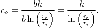(10.17)

Having obtained r_n, we would like to obtain the stress distribution in a curved beam with rectangular section subjected to a moment M. It follows from equation (10.15) that

σ = --y---∫-M---. rn - y a yda

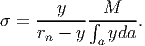(10.18)

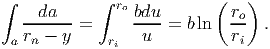
Now we need to compute ∫ _ayda with y measured from the neutral axis. Towards this,

∫ ∫ ro [ 1 ] yda = (rn - u)bdu = b rn(ro - ri) ---(r2o - r2i) = bh [rn - ρo], a ri 2

(10.19)

where we have used the fact that r_o - r_i = h and ρ_o = (r_o + r_i)∕2. Substituting equation (10.19) in (10.18), we obtain

M y σ = ---------------------------, bh (rn - y )[rn - (ri + ro)∕2]

(10.20)

where r_n - r_o ≤ y ≤ r_n - r_i. We compare the qualitative features of this solution after obtaining the elasticity solution.

10.3 2D Elasticity solution for curved beams

In this section, we obtain the two dimensional elasticity solution for the curved beam subjected to pure bending and end loading. The cross section of the beam is assumed to be rectangular of width 2b and depth h. As the beam is curved, we use cylindrical polar coordinates to formulate and study this problem. The curved beam is assumed to be the annular region between two coaxial radially cut cylinders of radius r_i and r_i + h, i.e, = {(r,θ,z)|r_i ≤ r ≤ r_o,α₁ ≤ θ ≤ α₂,-b ≤ z ≤ b}, where r_i, r_o, α₁, α₂ and b are constants. Note that here r_o = r_i + h

10.3.1 Pure bending

Figure 10.3: Curved beam subjected to pure bending

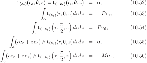
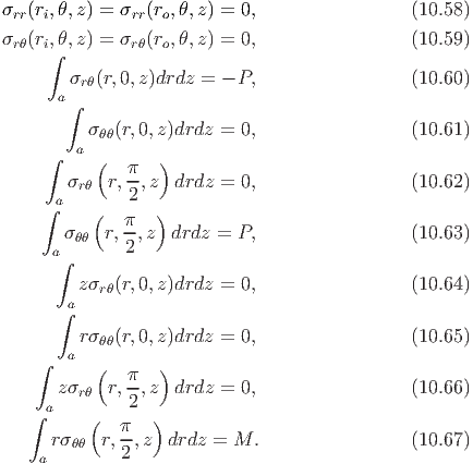
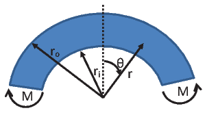
The first example that we study, is that of pure bending of a curved beam. Here the curved beam is assumed to be subjected to end moments as shown in figure 10.3. The traction boundary conditions for this problem are

The surfaces defined by r = r_i and r = r_o are traction free.
The surfaces defined by θ = ±α though is subjected to a moment, M along the z direction, has no net force.

Translating these boundary conditions into mathematical statements:

∫ t(er)(ro,∫θ,z) = t(-er)(ri,θ,z) = o, (10.21) t(eθ)(r,α,z)drdz = t(-eθ)(r,- α, z)drdz = o, (10.22) a ∫ a (rer + zez) ∧ t(e )(r,α, z)drdz = M ez, (10.23) a θ ∫ (rer + zez) ∧ t(-eθ)(r,- α, z)drdz = - M ez, (10.24) a

where {e_r,e_θ,e_z} are the cylindrical polar coordinate basis.

The displacement boundary condition for this problem are

The surface defined by θ = 0 undergoes no tangential displacement.
There is no radial displacement of the point with cylindrical polar coordinates (r_n, 0, 0), where r_n is the radial location on the surface θ = 0 at which σ_θθ(r_n, 0,z) = 0.

The mathematical statements of these conditions are

eθ ⋅ u (r,0,z) = 0, (10.25) er ⋅ u (rn,0,0) = 0. (10.26)

Assuming that the state of stress in the curved beam is plane and the cylindrical polar components of this stress are

( ) σrr σr θ 0 σ = ( σrθ σ θθ 0) . 0 0 0

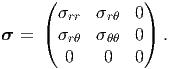(10.27)

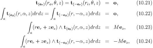
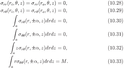
Substituting the above stress (10.27) in the traction boundary conditions (10.21) through (10.24) we obtain,

σrr(ri,θ,z) = σrr(ro,θ,z) = 0, (10.28) σrθ(ri,θ,z) = σrθ(ro,θ,z) = 0, (10.29) ∫ σrθ(r,± α,z)drdz = 0, (10.30) ∫a σθθ(r,± α,z)drdz = 0, (10.31) ∫ a zσ (r,± α,z)drdz = 0, (10.32) a rθ ∫ rσ θθ(r,± α,z )drdz = M. (10.33) a

Now, we have to find Airy’s stress function, ϕ that would satisfy the boundary conditions (10.28) through (10.33) and the bi-harmonic equation. In this problem we expect the stresses to be such that σ(r,θ,z) = σ(r,-θ,z), for any θ, i.e. the stress is an even function of θ. Imposing this restriction that the stress be an even function of θ, on the general periodic solution to the bi-harmonic solution (7.57), results in requiring that the Airy’s stress function be independent of θ. Thus, Airy’s stress function is,

ϕ = a01 + a02 ln (r) + a03r2 + a04r2ln(r),

(10.34)

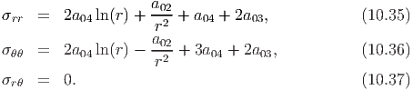
where the constants a_0i’s are to be found from the boundary conditions. The stress field corresponding to this Airy’s stress function, (10.34) found using (7.53) is

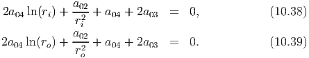
σrr = 2a04 ln (r) + a02 + a04 + 2a03, (10.35) r2 σ = 2a ln (r) - a02 + 3a + 2a , (10.36) θθ 04 r2 04 03 σrθ = 0. (10.37)

It can be immediately seen that by virtue of σ_rθ = 0, boundary conditions (10.29), (10.30) and (10.32) are trivially satisfied. The boundary condition (10.28) requires that

2a04 ln(ri) + a02+ a04 + 2a03 = 0, (10.38) r2i a02 2a04ln(ro) + r2 + a04 + 2a03 = 0. (10.39) o

The boundary condition (10.31) requires that

[ a02 ] [ a02 ] ro 2a04ln(ro) + -2-+ a04 + 2a03 - ri 2a04ln(ri) + --2 + a04 + 2a03 = 0. ro ri

(10.40)

By virtue of the terms in the square brackets being same as those in equations (10.39) and (10.38), equation (10.40) holds if (10.38) and (10.39) are satisfied. The only remaining boundary condition (10.33) when evaluated mandates that

( ) 2 2 ro 2 2 M-- a04[ro ln (ro) - ri ln(ri)] - a02ln r + (a04 + a03)(ro - ri) = 2b . i

(10.41)

Solving equations (10.38), (10.39) and (10.41) for the unknown constants a_0i’s, we obtain

( ) M 2 2 ro a02 = ---4riro ln -- , (10.42) N ri a = - M--[r2- r2+ 2(r2 ln(r ) - r2ln(r ))] , (10.43) 03 N o i o o i i M 2 2 a04 = ---2[ro - ri], (10.44) N

where

{ [ ( ) ] } 2 22 2 2 ro 2 N = 2b (ro - ri) - 4riro ln r . i

(10.45)

Substituting these constants from equation (10.42) through (10.44) in the expression for the stresses (10.35) through (10.37) the stress field becomes known.

(a) Beam with large initial curvature (b) Beam with moderate initial curvature

Figure 10.4: Comparison of the Winkler-Bach formula for the stress in the curved beams with the two dimensional elasticity solution for beams with different initial curvatures

(a) Beam with small initial curvature (b) Beam with negligible initial curvature

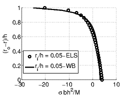
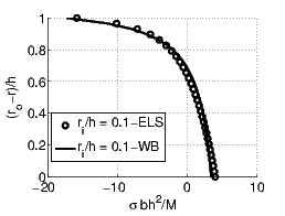
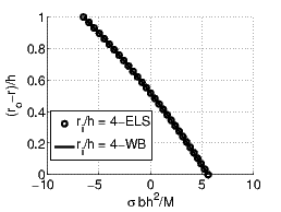
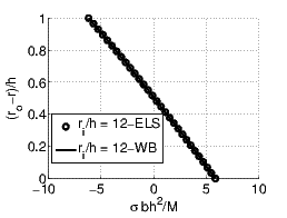
Figure 10.5: Study on the influence of initial curvature of the beam on the bending stresses developed due to a given moment

In figure 10.4 we compare the bending stress (σ_θθ) obtained using the Winkler-Bach formula with that obtained using the two dimensional elasticity approach. We find that both these approaches though predict different expressions for the stress, evaluate to the same values as seen from figure 10.4b. However, differences between these approaches increases as r_i∕h value tends to zero as seen from figure 10.4a.

In figure 10.5 we study when critical curvature of the beam above which the stresses in the beam are not influenced much by the curvature. It seems that if the curvature of the innermost fiber exceeds 5 times the depth of the beam with rectangular cross section, one can consider the beam as straight for practical purposes.

Having obtained the stress field that satisfies the compatibility conditions, a smooth displacement field corresponding to this stress field can be determined by following the standard approach of estimating the strains for this stress field from the two dimensional constitutive relation and then integrating the resulting strains for the displacements using the strain displacement relation. On performing these calculations, we find that the cylindrical polar components of the displacement field are given by

[ ( )]
ur = 1- 2(1 - ν)(a04r ln (r) + a03r) - (1 + ν) a02+ a04r
E r
+ C1 sin(θ) + C2cos(θ),

(10.46)

4a04- uθ = E rθ + C1 cos(θ ) - C2 sin(θ) + C3r,

(10.47)

where C_i’s are constants to be determined from the displacement boundary conditions, u_r is the radial component of the displacement and u_θ is the tangential component of the displacement.

Substituting equation (10.47) in the displacement boundary condition (10.25) we obtain,

C1 + C3r = 0.

(10.48)

For equation (10.48) to hold,

C1 = 0, C3 = 0.

(10.49)

In order to satisfy the displacement boundary condition (10.26),

[ ( ) ] -1 a02 C2 = - E 2(1 - ν)(a04rnln(rn) + a03rn) - (1 + ν) r + a04rn . n

(10.50)

10.3.2 Curved cantilever beam under end load

Figure 10.6: Curved cantilever beam subjected to end loading

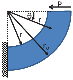
The next example that we study, is that of end loading of a curved cantilever beam. Here a cantilever beam is assumed to be subjected to end shear force as shown in figure 10.6. Thus, the displacement boundary condition for this problem is

The surface defined by θ = undergoes no displacement.

The mathematical statement of this condition is

π u(r,--,z) = o, 2

(10.51)

The traction boundary conditions for this problem are

The surfaces defined by r = r_i and r = r_o are traction free.
The surface defined by θ = 0 is subjected to a force, -P along the radial direction.
The surface defined by θ = , is subjected to a force, P along tangential direction and to a moment M along the z direction. The value of this moment M needs to be determined so that the required displacement boundary conditions are satisfied.

Translating these boundary conditions into mathematical statements:

t(er)(ro,θ,z) = t(-er)(ri,θ,z) = o, (10.52) ∫ t(eθ)(r,0,z )drdz = - P er, (10.53) ∫ a ( π- ) t(- eθ) r,2 ,z drdz = Peθ, (10.54) ∫ a (rer + zez) ∧ t(e )(r,0,z )drdz = o, (10.55) a θ ∫ ( π ) (rer + zez) ∧ t(- eθ) r,--,z drdz = - M ez, (10.56) a 2

where {e_r,e_θ,e_z} are the cylindrical polar coordinate basis.

Assuming that the state of stress in the curved beam is plane and the cylindrical polar components of this stress are

( σrr σr θ 0) ( ) σ = σrθ σ θθ 0 . 0 0 0

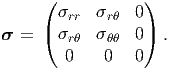(10.57)

Substituting the above stress (10.57) in the traction boundary conditions (10.52) through (10.56) we obtain,

σrr(ri,θ,z) = σrr(ro,θ,z) = 0, (10.58) σrθ(ri,θ,z) = σrθ(ro,θ,z) = 0, (10.59) ∫ σrθ(r,0,z)drdz = - P, (10.60) a∫ aσ θθ(r,0,z)drdz = 0, (10.61) ∫ ( π ) σrθ r,-,z drdz = 0, (10.62) ∫ a 2 ( π- ) σ θθ r,2 ,z drdz = P, (10.63) a∫ zσrθ(r,0,z)drdz = 0, (10.64) a ∫ rσ θθ(r,0,z)drdz = 0, (10.65) ∫ a ( ) π- a zσrθ r,2,z drdz = 0, (10.66) ∫ ( π ) rσθθ r,--,z drdz = M. (10.67) a 2

In order to satisfy the traction boundary conditions (10.58) through (10.67), we chose Airy’s stress function from the general solution (7.57) such that it contains only the sin(θ) and cos(2θ) terms as,

[ b ]
ϕ = b11r + b12r ln(r) + -13-+ b14r3 sin(θ)
r [ ]
2 4 a23
+ a21r + a22r + r2 + a24 cos(2θ).

(10.68)

To proceed further, one has to follow the standard procedure and hence, we leave it as an exercise to find the stress and displacement field.

10.4 Summary

In this chapter we studied on how to analyze beams with initial curvature. We obtained the stress field based on the assumption that the plane section remain plane after bending. We also obtained two dimensional elasticity solution which is not based on the assumption that plane sections remain plane. However, we found that both these solutions predict the same value of stresses for practically used curved beams.

10.5 Self-Evaluation

There are two beams - a straight beam and a curved beam - each of which is subjected to a pure bending moment, M. Assuming that both the beams are homogeneous and has a square cross section with side 0.3m and are made of the same material, which is linear elastic and isotropic, compute the ratio of the maximum tensile stresses experienced in the straight and curved beams. Also, find the ratio of the maximum compressive stresses experienced in the straight and curved beams. Assume, the curved beam forms a part of a circle, with the initial radius of curvature of the center line of the bar, being ρ_o. Obtain the value of the ratios as a function of ρ_o and determine the critical rho_o^c below which the stresses would differ by more than 10 percent.
A curved beam with a circular center line has the T-section as shown in figure 10.7. This beam is subjected to pure bending in its plane of symmetry. Find the tensile and compressive stresses in the extreme fibers. Assume, b₁ = 100 mm, b₂ = 20 mm, the radius of curvature of the innermost fiber, r₁ = 80 mm, the outermost fiber, r₂ = 180 mm and r₃ = 100 mm.
A curved beam with a circular center line has the circular sections as shown in figure 10.8. Find the stress distribution across this section if the curved beam is subjected to a pure bending moment, M. Assume that the initial curvature of the center line of the beam is ρ_o.

Figure 10.7: T section. Figure for problem 2

Figure 10.8: Circular section. Figure for problem 3

[prev] [prev-tail] [front] [up]

Chapter 10Bending of Curved Beams