Delay analysis at signalized intersection
To begin with assume that the arrival process is deterministic and vehicle arrive at a uniform rate. Further, assume that the system in unsaturated, that is, the total number of vehicles that arrive in a period is less than the total number of vehicles that can be served by the system. These two assumptions mean that the arrival rate is such that all the vehicles that come in a cycle are cleared within the same cycle (like the situation in Cycle I of Figure 7).
The average delay to vehicles for this case can then be easily determined from the figure shown in Figure 8. The figure shows a typical cumulative arrival/departure graph against time for an unsaturated, uniform arrival rate approach to an intersection. The slope of the cumulative arrival line is  , where is the uniform arrival rate in vehicles per unit time. The slope of the cumulative departure line is sometimes zero (when the light is red) and sometimes , where is the uniform arrival rate in vehicles per unit time. The slope of the cumulative departure line is sometimes zero (when the light is red) and sometimes  (when the light is green); where is the saturation flow rate obtained as the reciprocal of the saturation headway explained earlier; is expressed as vehicles per hour of green per lane or vphgpl. (when the light is green); where is the saturation flow rate obtained as the reciprocal of the saturation headway explained earlier; is expressed as vehicles per hour of green per lane or vphgpl.
Fig. 8: A typical plot of cumulative number of arrivals and departures on an unsaturated, uniform arrival rate approach to a signalized intersection.
|
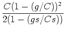
From the figure 8 (where C is the duration of the cycle length and g the duration of the effective green period) it can be seen that the total delay (under the assumptions stated above),  , is given by , is given by
Assuming that n is large enough so that the discrete sum of d(i) is equal to the area of the triangle in the figure, the following can be written:
From the figure,  can be easily determined by noting that can be easily determined by noting that
where,
Determining  from the above relation, can be written as from the above relation, can be written as
Hence,
From the above and noting that n, the total number of vehicles that arrived, is C the average delay under the above assumptions,  , can be obtained as: , can be obtained as:
However, an approach to an intersection may not always stay unsaturated. There may be periods of over-saturation during which the arrivals from one cycle spill over to the next and so on. A similar situation can be seen in Cycle II of Figure 7. Under this assumption, and the assumption that arrival rate is still deterministic and uniform, the plot of cumulative arrivals/departures versus time can be drawn (see Figure 8). In the figure it is assumed that the arrival rate from 0 to time T is , and that is large enough to cause oversaturation (i.e., C greater than sg, the maximum number of vehicles that can be served during a cycle).
Fig. 9: A typical plot of cumulative number of arrivals and departures on an over-saturated, uniform arrival rate approach to a signalized intersection.
|
From the figure 9 it can be seen that the total delay under these assumptions, i.e.  , is given by the sum of the area marked with horizontal stripes (Area I) and the area marked with inclined stripes (Area II). This implies that the average delay, i.e. , is given by the sum of the area marked with horizontal stripes (Area I) and the area marked with inclined stripes (Area II). This implies that the average delay, i.e.  , under these assumptions is the sum of the average delay due to Area I and the average delay due to Area II. , under these assumptions is the sum of the average delay due to Area I and the average delay due to Area II.
The average delay due to Area II can be easily determined by assuming the dashed line as the cumulative arrival line and using Equation 9. However, first the slope of the dashed line needs to be determined and later substituted for in Equation 9. If the slope of the dashed line is taken as  (and noting that the slope of the inclined part of the cumulative departure line is , the saturation flow rate) then (and noting that the slope of the inclined part of the cumulative departure line is , the saturation flow rate) then

or
Substituting this expression of for in Equation 9 we can write the average delay due to Area II,  , as , as
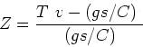
The average delay due to Area I can be determined by looking at the average time between the cumulative arrival line and the dashed line. If the horizontal distance (i.e., time in this case) between Point P and the dashed line is taken as Z, then it can be said that the time between the cumulative arrival line and the dashed line increases linearly from 0 to Z over a time period of 0 to T. From this it can be said that the average delay for vehicles arriving between time 0 and T is Z/2 (Note that the area of the triangle formed by the cumulative arrival line, a horizontal line from P and the dashed line is given by Zn/2, where  is the number of vehicles to arrive till time T). is the number of vehicles to arrive till time T).
Similarly, the time between the cumulative arrival line and the dashed line decreases linearly from Z to 0 over a time period of T to M. Following the same logic as above, the average delay due to Area I to vehicles arriving between times T and M is Z/2. Hence, it can be said that the average delay due to Area I is Z/2 irrespective of when a vehicle arrives.
If one assumes the vertical distance of Point P from the dashed line as y, then
 = Slope of the dashed line, σ = Slope of the dashed line, σ
and
hence,
 |
(11) |
or
where,  , represents the maximum number of vehicles that can cross the intersection from a given approach per unit time. , represents the maximum number of vehicles that can cross the intersection from a given approach per unit time.
Thus the average delay, is given as
In reality, however, more often than not the arrival is not deterministic, it is stochastic. Once it is assumed that the arrival is stochastic the above relations cannot be used and can at best function as approximate estimates. Assumption of stochastic arrivals lead us to analysis which is beyond the scope of this section. Hence, in this text, only the relations generally used to determine delay under the above assumptions are described.
One of the relations often used in determining delay is due to Webster [259]. Webster assumed that the arrivals are according to a Poisson distribution, departures occur uniformly and at a maximum rate of , the average arrival rate is such that  , and that the queueing process runs under similar arrival and departure conditions long enough for the system to stabilize to a steady state (where, for example, cycle to cycle variations in average delay, average queue length, etc. are minimal). Based on these assumptions and some simulation runs (where the arrival and departure processes at a signalized intersection are simulated for various arrival pattern and signal settings) Webster proposed the following expression for average delay, , and that the queueing process runs under similar arrival and departure conditions long enough for the system to stabilize to a steady state (where, for example, cycle to cycle variations in average delay, average queue length, etc. are minimal). Based on these assumptions and some simulation runs (where the arrival and departure processes at a signalized intersection are simulated for various arrival pattern and signal settings) Webster proposed the following expression for average delay,  : :
 |
(13) |
The first term in the equation is the same as that given in Equation 9, the second term is the additional term which results from analyzing the process by assuming stochastic arrivals, the third term is a correction factor obtained from simulation studies. It is seen that this term is often between 5 and15 per cent of the sum of the first two terms. Hence the following simplified form of the above equation is sometimes used.
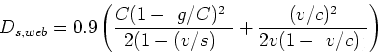
In practice, it is found that the estimates of delay are not good for the entire range of /C values. In general, when /C values are close to one (that is, C is close to  , this implies an increase in the chances of oversaturation when the stochasticity in the arrival rate causes the number of arrivals to be greater than ), overestimates the average delay. One possible reason for this is that the derivation of the quantity assumes steady-state behaviour, which is never achieved at real intersections as oversaturation by design occurs only in short spells. Other researchers around the world have developed other equations which are supposed to predict delays more realistically. All of them predict values which are close to when /C is not high (say less than 0.8) while their estimates are much lower when /C is high (say greater than 0.95). The 1985 Highway capacity manual of USA [104] proposes the use of one such expression for delay, , this implies an increase in the chances of oversaturation when the stochasticity in the arrival rate causes the number of arrivals to be greater than ), overestimates the average delay. One possible reason for this is that the derivation of the quantity assumes steady-state behaviour, which is never achieved at real intersections as oversaturation by design occurs only in short spells. Other researchers around the world have developed other equations which are supposed to predict delays more realistically. All of them predict values which are close to when /C is not high (say less than 0.8) while their estimates are much lower when /C is high (say greater than 0.95). The 1985 Highway capacity manual of USA [104] proposes the use of one such expression for delay,  , reproduced here as Equation 14. The relation was developed based on a large database on intersection delay. , reproduced here as Equation 14. The relation was developed based on a large database on intersection delay.
![\begin{displaymath}
D_{s,hcm85}=0.76\frac{C(1-(g/C))^2}{2(1-(v/s))} + 173(v/c)^2 \left[ ((v/c)-1)
+ \sqrt{((v/c)-1)^2 + 16(v/c^2)} \right]
\end{displaymath}](img133.png) |
(14) |
The 1985 HCM [104] cautions users against using this relation for  . In the 1998 HCM [103] the calculation of delay has been further modified. That expression is not provided here as it uses many site specific empirical constants which are not valid for Indian conditions. . In the 1998 HCM [103] the calculation of delay has been further modified. That expression is not provided here as it uses many site specific empirical constants which are not valid for Indian conditions.
|