Example for signalized intersection
On an approach to a signalized intersection, the effective green time and effective red time are 30 s each. The arrival rate of vehicles on this approach is 360 vph between 0-120 s; 1800 vph between 120-240 s, and 0 vph between 240-420 s. The saturation flow rate for this approach is 1440 vphgpl. The approach under consideration has one lane. Assume that at time = 0 s the light for the approach has just turned red.
- Plot the arrival rate of vehicles versus time.
- Assuming arrival and departure processes to be continuous, plot the cumulative number of arrivals and departures versus time.
- Determine the average delay to vehicles arriving between 0-120 s.
- Determine the average delay to vehicles arriving between 120-240 s.
- Determine the average delay to vehicles arriving between 0-240 s.
- Determine the delays to the fourth and the sixtieth vehicles that arrive at the intersection.
- Determine the maximum delay faced by a vehicle on this approach.
- Determine the maximum queue length on this approach. At what time does the queue length first become equal to the maximum?
- Determine the percentage of time for which there exists a queue on this approach.
- Determine the average queue length between 120 and 420 s.
Solution
The following parameter values are provided:g = 30 s, C = 30 + 30 = 60 s , s = 1440 vphgpl,  from 0-120 s = 360 vph, from 120-240 s = 1800 vph, and from 240-420 s = 0 vph, and T, the time for which there exists a flow higher than from 0-120 s = 360 vph, from 120-240 s = 1800 vph, and from 240-420 s = 0 vph, and T, the time for which there exists a flow higher than  , is 120 s. Note, c = (g/C)s= 720 vph. , is 120 s. Note, c = (g/C)s= 720 vph.
(i) Figure 14 gives the plot of arrival rate of vehicles versus time.
(ii) Figure15 gives the plot of cumulative arrivals and departures versus time.
(iii) Between 0-120 s the intersection is operating under unsaturated conditions. Further, the arrival is deterministic and uniform. Hence we can use Eq 9 to determine the average delay. Therefore,
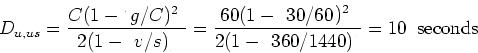
Fig. 14: Plot of arrival rate versus time.
 |
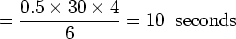
We can also determine the average delay directly from the graph, by noting that the area of either Triangle I or Triangle II in Figure 16 (which is the same as Figure 15 but with few extra annotations) divided by the total number of arrivals during a cycle will give the average delay. Therefore,
Average delay = Area of Triangle I or II
Number of arrivals in a cycle
 (iv) Between 120-240 s the intersection is operating under oversaturated conditions. The arrival is deterministic and uniform. Hence we can use Equation 12 to determine the average delay. Thus,
We can also determine the average delay directly from the graph (see Figure16), by noting that,
Fig. 15: Plot of cumulative number of arrivals and departures of vehicles versus time.
(v) The average delay to all the vehicles between 0-240 s can be obtained by dividing the total delay (faced by all vehicles) by the total number of vehicles. Hence,
where,  is the number of vehicles that arrive during 0-120 s is the number of vehicles that arrive during 0-120 s
 is the average delay to a vehicle coming during 0-120 s is the average delay to a vehicle coming during 0-120 s
 is the number of vehicles that arrive during 120-240 s is the number of vehicles that arrive during 120-240 s
 is the average delay to a vehicle arriving during 120-240 s. is the average delay to a vehicle arriving during 120-240 s.
Hence,
Of course, we can also find the average delay here from the graph (the reader should do this).
(vi) The arrival rate of vehicles from 0 to 120 seconds is 360 vph or 0.1 vps. Assuming that the fourth vehicle arrives before 120 seconds, the time of arrival of the fourth vehicle is 4/0.1 = 40 seconds. (Hence the assumption is not violated).
The departure rate of vehicles is 1440/3600 = 0.4 vps. The time of departure of the fourth vehicle, assuming that the fourth vehicle gets discharged during the first green, is 30 + 4/0.4 = 40 s. (Since the departure time is less than the start of the next red, the assumption is valid.)
The delay to the fourth vehicle therefore is
departure time - arrival time = 40 -40 = 0 s
The same observation can be made from Figure 16. 
Fig 16. Example: Plot of cumulative number of arrivals and departures of vehicles versus time.
The delay to the sixtieth vehicle can also be read from Figure 16 as 144 seconds.
(vii) As can be seen from the Figure 16 the maximum delay is 180 seconds.
(viii) As can be seen from Figure 16 the maximum queue length is 36 vehicles. At time = 240 s, the queue length first becomes equal to 36 vehicles.
(ix) As can be seen from Figure 16 there are no queues from 40-60 s and from 100-120 s. For the rest of the time, there is a queue at the intersection. Hence, the percentage of time for which there is no queue at the intersection is (40/420)100 = 9.52. Hence the percentage of time when there exists a queue is
. 100 - 9.52 = 90.48%
(x) We can determine the average queue length directly from Figure 16, by noting that,
|