|
At signalized intersections, other than collecting data on arrival rate and pattern (which can be done in the usual manner of counting volume and recording time headways), data on delay and saturation flow rates may need to be collected. In this section, procedures for collecting data on delay and saturation flow rates are described.
Collecting data on average delay
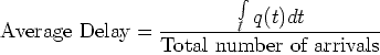
In this section a procedure which can be easily used to collect data on stopped delay at a signalized intersection is described. The procedure relies on the principle that the area between the cumulative arrival and departure plots (see figure 7) gives the total time that all the vehicles spend stopped at the intersection; its unit is vehicle seconds. This area divided by the total number of arrivals obviously gives the average delay.
The area can be obtained by summing either all the delays or all the queue lengths, that is,
Total area between cumulative arrivals and departure plots 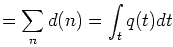
where all the variables are as explained in figure 7
Hence the average delay can be obtained as
The data collection procedure uses the above relation to evaluate the average delay. The method relies on determining the area by observing the queue lengths at short intervals of time over the entire experiment time period, and counting the total number of vehicles during the entire test period. The procedure is explained step-by-step as follows:
Step 1. Decide the time period P for which the data will be collected. Decide the interval of time I at which, the queue length at the intersection will be counted. The cycle length C should not be an integral multiple of I. Let the number of intervals in P be m.
Step 2. Count the queue length qi at the end of each interval. Continue counting till P is over. Also over the time P, count the total number of vehicles that arrive at the intersection, i.e.
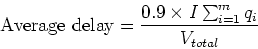
Step 3. Estimate the area as  . See Figure13, which is a figure similar to Figure 7. The area obtained using is generally seen to be more than the actual area, and hence the estimate obtained here is reduced by 10% in order to get a closer estimate of the true area. . See Figure13, which is a figure similar to Figure 7. The area obtained using is generally seen to be more than the actual area, and hence the estimate obtained here is reduced by 10% in order to get a closer estimate of the true area.
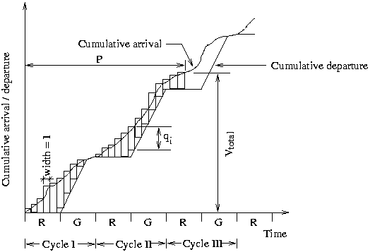
Fig.13
Step 4. Estimate the average delay as
Collecting data on saturation flow rate
The saturation flow rate is the reciprocal of the saturation headway. The saturation headway, as suggested in the subsection on DEPARTURE PROCESS, is the headway at which latter vehicles discharging from a queue cross the stop line. In general, the HCM [103] suggests that the average value of the saturation headway si for sample i can be obtained using
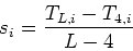
where Tj,i is the time at which the jth vehicle of the queue crosses the stop line for the ith sample, and L stands for the last vehicle in the queue. The assumption here is that from the fourth vehicle onwards all vehicles more or less maintain the saturation headway. According to the HCM [103], the average value of the saturation headway should be estimated as the mean of all  s after repeated sampling. s after repeated sampling.
|