When information is available on the growth in the number of trips originating
and terminating in each zone, we know that there will be different growth rates
for trips in and out of each zone and consequently having two sets of growth
factors for each zone.
This implies that there are two constraints for that model and such a model is
called doubly constrained growth factor model.
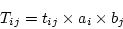
One of the methods of solving such a model is given by Furness who introduced
balancing factors  and and  as follows: as follows:
 |
(1) |
In such cases, a set of intermediate correction coefficients are calculated
which are then appropriately applied to cell entries in each row or column.
After applying these corrections to say each row, totals for each column are
calculated and compared with the target values.
If the differences are significant, correction coefficients are calculated and
applied as necessary.
The procedure is given below:
- Set = 1
- With solve for to satisfy trip generation constraint.
- With solve for to satisfy trip attraction constraint.
- Update matrix and check for errors.
- Repeat steps 2 and 3 till convergence.
Here the error is calculated as:
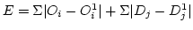 where where  corresponds to
the actual productions from zone corresponds to
the actual productions from zone  and and  is the calculated productions
from that zone. Similarly is the calculated productions
from that zone. Similarly  are the actual attractions from the zone are the actual attractions from the zone  and
and  are the calculated attractions from that zone. are the calculated attractions from that zone.
|