| |
| | |
|
The difference between the earlier model and this model is the number of
servers.
This is a multi -server model with N number of servers whereas the earlier one
was single server model.
The assumptions stated in M/M/1 model are also assumed here.
Figure 1:
Multi-server model
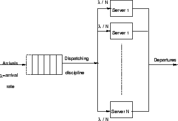 |
Here  is the average service rate for N identical service counters in
parallel.
For x=0 is the average service rate for N identical service counters in
parallel.
For x=0
![$\displaystyle P(0)=\left[\sum_{x=0}^{N-1}\left(\frac{\rho^x}{x!}+\frac{\rho^N}{(N-1)!(N-\rho)}\right)\right]^{-1}$](img3.png) |
(1) |
The probability of x number of customers in the system is given by P(x).
For

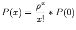 |
(2) |
For 
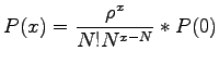 |
(3) |
The average number of customers in the system is
![$\displaystyle E[X] = \rho+[\frac{\rho^{N+1}}{(N-1)!(N-\rho)^2}]P(0)$](img8.png) |
(4) |
The average queue length
![$\displaystyle E[L_q] = [\frac{\rho^{N+1}}{(N-1)!(N-\rho)^2}]P(0)$](img9.png) |
(5) |
The expected time in the system
![$\displaystyle E[T] = \frac{E[X]}{\lambda}$](img10.png) |
(6) |
The expected time in the queue
![$\displaystyle E[T_q] = \frac{E[L_q]}{\lambda}$](img11.png) |
(7) |
Consider the earlier problem as a multi-server problem with two servers in
parallel.
Average arrival rate =  = 300 vehicles/hr.
Average service rate = = 300 vehicles/hr.
Average service rate =
 vehicles/hr.
Utilization factor = traffic intensity = vehicles/hr.
Utilization factor = traffic intensity =
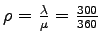 = 0.833. = 0.833.
Average number of vehicles in the system is = L =
![$ E[X]=
\rho+[\frac{\rho^{N+1}}{(N-1)!(N-\rho)^2}]P(0)$](img19.png) = 1.22.
The average number of customers in the queue = = 1.22.
The average number of customers in the queue =
![$ L_q = E[L_q] =
[\frac{\rho^{N+1}}{(N-1)!(N-\rho)^2}]P(0)$](img20.png) = 0.387.
Expected time in the system = = 0.387.
Expected time in the system =
![$ W = \frac{E[X]}{\lambda}$](img21.png) = 0.004 hr = 14 sec.
The expected time in the queue = = 0.004 hr = 14 sec.
The expected time in the queue =
 = 0.00129 hr = 4.64
sec. = 0.00129 hr = 4.64
sec.
|
|
| | |
|
|
|
![$\displaystyle \left[\sum_{x=0}^{N-1}\left(\frac{\rho^x}{x!}+\frac{\rho^N}{(N-1)!(N-\rho)}\right)\right]^{-1}$](img17.png)