Module 8 : Specialized Traffic Studies

Lecture 45 : Queuing Analysis

1

2

3

4

5

6

7

8

	System performance measures The following notation assumes that the system is in a steady-state condition (At a given time t): Utilization factor $\rho = \frac{\lambda}{\mu}$ Pn = probability of exactly n customers in queuing system (waiting + service). L= expected(avg) number of customers in queuing system. [sometimes denoted as Ls] Lq=expected (avg) queue length (excludes customers being served) or no of Customers. W = Expected waiting time in system (includes service time) for each individual customer or time a customer spends in the system. [sometimes denoted as Ws] Wq = waiting time in queue (excludes service time) for each individual customer or Expected time a customer spends in a queue Relationships between L, W, Lq and Wq: Assume that $\lambda_n$ is a constant $\lambda$ for all n. It has been proved that in a steady-state queuing process, ($\lambda$ may be considered as avg): $L = \lambda W$ $Lq = \lambda Wq$ $W = Wq + \frac{1}{\lambda}$ Queuing Patterns A variety of queuing patterns can be encountered and a classification of these patterns is proposed in this section. The classification scheme is based on how the arrival and service rates vary over time. 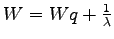In the following figures the top two graphs are drawn taking time as independent variable and volume of vehicles as dependant variable and the bottom two graphs are drawn taking time as independent variable and cumulative volume of vehicles as dependant variable. Constant arrival and service rates Figure 1: Constant arrival and service rates In the left hand part of the Fig.1 arrival rate is less than service rate so no queuing is encountered and in the right hand part of the figure the arrival rate is higher than service rate, the queue has a never ending growth with a queue length equal to the product of time and the difference between the arrival and service rates. 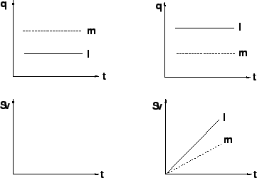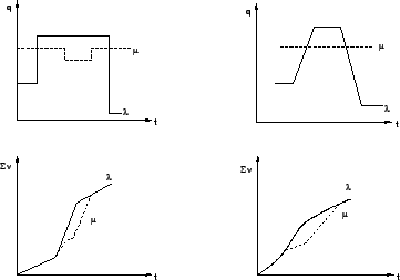Constant arrival rate and varying service rate Figure 2: Constant arrival rate and varying service rate In the left hand of Fig. 2 the arrival rate is constant over time while the service rates vary over time. It should be noted that the service rate must be less than the arrival rate for some periods of time but greater than the arrival rate for other periods of time. One of the examples of the left hand part of the figure is a signalized intersection and that of the right hand side part of the figure is an incident or an accident on the roads which causes a reduction in the service rate. 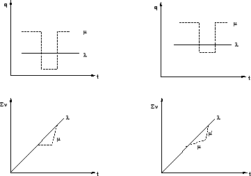Varying arrival rate and constant service rate Figure 3: Varying arrival rate and constant service rate In the left part of Fig. 3 the arrival rate vary over time but service rate is constant. Both the left and right parts are examples of traffic variation over a day on a facility but the left hand side one is an approximation to make formulations and calculations simpler and the right hand side one considers all the transition periods during changes in arrival rates. 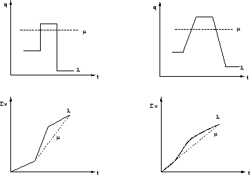Varying arrival and service rates Figure 4: Varying arrival and service rates In the Fig.4 the arrival rate follows a square wave type and service rate follows inverted square wave type. The diagrams on the right side are an extension of the first one with transitional periods during changes in the arrival and service rates. These are more complex to analyzed using analytical methods so simulation is often employed particularly when sensitivity parameter is to be investigated.