|
Air Pollution Models give a causal relationship between emissions, meteorology,
atmospheric concentrations, deposition, and other factors.
They explain the consequences of past and future scenarios and the
determination of the effectiveness of abatement strategies.
They are also used to describe the concentration of various pollutants in the
air.
The major types of air pollution models are emission models and dispersion
models.
Emission models are commonly used to provide traffic emission information for
the prediction and management of air pollution levels near roadways.
The model helps in comparing the actual pollution levels with the emission
standards set.
Hence, the abatement of pollution can also be carried out.
The basic schematic diagram of an emission model is given in the
Fig. 1.
Figure 1:
Basic Schematic Diagram of an Emission model
![\begin{figure}
\centerline{\epsfig{file=qfFuelEmissionModel.eps,width=8cm}}
%, Source: [2]}
\end{figure}](img1.png) |
Emission models estimate the emission quantity using the emission factor.
The emission factor may be defined as the ratio of average amount of pollutant
discharged to the total amount of the fuel discharged.
It is expressed in kg of particulate / metric ton of fuel.
The emission factors used in the emission models reflect different levels of
congestion.
The various types of emission models are briefly discussed in the following
paragraphs.
The model is similar to the instantaneous fuel consumption model.
It describes the vehicle emission behavior during any instant of time.
The advantages of the model are that the emission factors can be calculated and
generated for any vehicle operating profile, and the model considers dynamics
in driving patterns.
The model has some disadvantages also such as:
Detailed and precise information on vehicle operation and location is required
and
The process of data collection is expensive.
This model is useful in macro level where detailed information is not required.
A single emission factor is used to represent a particular type of vehicle and
general type of driving.
Emission is estimated using the equation:
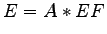 |
(1) |
where,  = emissions, in units of pollutant per unit of time, = emissions, in units of pollutant per unit of time,  = activity
rate, in units of weight, volume, distance or duration per unit of time, = activity
rate, in units of weight, volume, distance or duration per unit of time,  =
emission factor, in units of pollutant per unit of weight, volume, distance or
duration
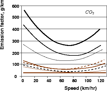
The variation of exhaust emission factors with speed for the major exhaust
pollutants are given in the following figures
(Fig. 2 to Fig. 7). =
emission factor, in units of pollutant per unit of weight, volume, distance or
duration
The variation of exhaust emission factors with speed for the major exhaust
pollutants are given in the following figures
(Fig. 2 to Fig. 7).
file=qfFuelCommon.eps,width=8cm
Figure 2:
Variation of emission factor with Speed for Particulate Matter
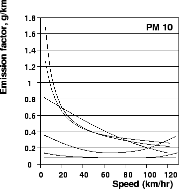 |
Figure 3:
Variation of emission factor with Speed for Nitrogen Oxides
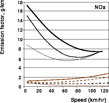 |
Figure 4:
Variation of emission factor with Speed for Volatile Organic
Compounds
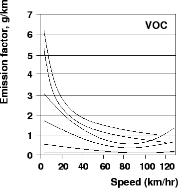 |
Figure 5:
Variation of emission factor with Speed for Carbon Monoxide, Source:
[5]
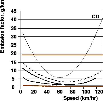 |
Figure 6:
Variation of emission factor with Speed for Sulphur Dioxide
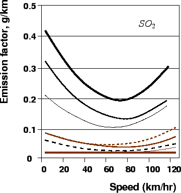 |
Figure 7:
Variation of emission factor with Speed for Carbon Dioxide
 |
For Particulate Matter  and Volatile Organic Compounds, the emissions
steadily decrease with the speed.
In case of Nitrogen Oxides, Sulphur Oxides and Carbon Dioxide, the emission is
highest for low speeds, decreases for intermediate speeds and then again
increases with the speed.
For Carbon Monoxide, the highest emission levels occur for higher speeds and
minimum emission occurs for intermediate speeds.
Using the emission factor model, the amount of CO emitted by a vehicle was
estimated as 50 grams per hour.
If the vehicle travelled at a velocity of 40kmph, estimate the emission factor
for CO for the vehicle.
It is given that the total emission is 50g/hr.
The activity ‘’ here is the amount of and Volatile Organic Compounds, the emissions
steadily decrease with the speed.
In case of Nitrogen Oxides, Sulphur Oxides and Carbon Dioxide, the emission is
highest for low speeds, decreases for intermediate speeds and then again
increases with the speed.
For Carbon Monoxide, the highest emission levels occur for higher speeds and
minimum emission occurs for intermediate speeds.
Using the emission factor model, the amount of CO emitted by a vehicle was
estimated as 50 grams per hour.
If the vehicle travelled at a velocity of 40kmph, estimate the emission factor
for CO for the vehicle.
It is given that the total emission is 50g/hr.
The activity ‘’ here is the amount of  emitted by the vehicle, which is
40km/hr. from the eqn. 1, we have, the total emissions is emitted by the vehicle, which is
40km/hr. from the eqn. 1, we have, the total emissions is
 .
Therefore, the emission factor will be .
Therefore, the emission factor will be  = 50/40 = 1.25.
That is, the emission factor of is 1.25 grams/km. = 50/40 = 1.25.
That is, the emission factor of is 1.25 grams/km.
|
|