Module 8 : Specialized Traffic Studies

Lecture 43 : Fuel Consumption and Emission Studies

1

2

3

4

5

6

7

8

9

10

11

12

	Drive Mode Elemental Model Unlike the average speed model, the drive model elemental model is a microscopic fuel consumption model. It considers the movement of a single vehicle. This model is used to obtain the fuel consumption rates during various vehicle operating conditions or drive mode. The different drive modes include cruising, idling, accelerating and decelerating, which together form a driving cycle. The important assumptions used in this model are that the driving mode elements are independent of each other and the sum of the component consumption equals the total amount of fuel consumed. The advantages of this model are that the model is simple and general and there is a direct relationship to existing traffic modelling techniques. The disadvantage of this model is that the variation in the behavior of different drivers and behavior of the same driver under different situations is ignored.The component elements considered here are various drive modes such as cruising, idling and accelerating. The total fuel consumed for the drive mode elemental model is given by the relation: 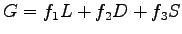$$G = f_1L+f_2D+f_3S$$ (1) where, $G$ = fuel consumed per vehicle over a measured distance (total section distance), $L$ = total section distance traveled, $D$ = stopped delay per vehicle (time spent in idling), $S$ = number of stops, $f_1$ = fuel consumption rate per unit distance while cruising, $f_2$ = fuel consumption rate per unit time while idling, $f_3$ = excess fuel used in decelerating to stop and accelerating back to cruise speed Numerical example The total fuel consumption by a vehicle travelling on a stretch of road is 0.0735 liters/veh-km. The average stopped delay for the vehicle is 6s. The vehicle stops thrice during its journey. Assume $f_1$ = 0.0045, $f_2$ = 0.0035 and $f_3$ = 0.002. Calculate the length of road considered. If the vehicle is cruising throughout the stretch of the road, what is the decrease in fuel consumption? Solution: From the equation. 1, the fuel consumed per vehicle over a measured distance is given by $$G = f_1L+f_2D+f_3S$$ Step 1:  It is given that fuel consumed per vehicle is 0.0735 liters/veh-km, average delay is 6s and the number of stops are 3. The values of $f_1$, $f_2$ and $f_3$ are given as 0.0045,0.0035 and 0.002 respectively. It is required to find the length of the road. The length L can be computed from the above equation as given: $0.0735 = (0.0045 * L) + (0.0035 * 6) + (0.002 * 3)$. Therefore, Length, $L$ is equal to 10 km. Step 2:  When the vehicle is cruising throughout the length, there will not be any delays or stops. Therefore, total fuel consumption: $G’ = f_1L = 0.0045 * 10 = 0.045 liters/veh-km$. Step 3:  The decrease in fuel consumption is will be the difference in fuel consumptions as obtained in steps 1 and 2, which is 0.0735-0.045 = 0.0285 liters/veh-km. Instantaneous Model Instantaneous fuel consumption models are derived from a relationship between the fuel consumption rates and the instantaneous vehicle power. Second-by-second vehicle characteristics, traffic conditions and road conditions are required in order to estimate the expected fuel consumption. Due to the disaggregate characteristic of fuel consumption data, these models are usually implemented to evaluate individual transportation projects such as single intersections, toll plazas, sections of highway, etc. In this model the fuel consumption rate is taken as the function of different variables such as weight of vehicle, drag coefficient, rolling resistance, frontal area, acceleration and speed, transmission efficiency and grade.