Consider an intersection of two streets with a single lane in each direction.
Each approach has identical characteristics and carries 675 veh/h with no left
or right turns.
The average headway is 2.0 s per vehicle and the lost time per phase is 3.0 s.
Detectors are 9.1 m long with no setback from the stop line.
The actuated controller settings are as follows:
| Setting |
Time (s) |
| Initial interval |
10 |
| Unit extension |
3 |
| Maximum green |
46 |
| Intergreen |
4 |
Determine the phase time for this intersection with actuated controller for
approach speed 50 kmph.
The maximum phase time for each phase will be (46 + 4) = 50 s.
The minimum phase time will be 10 + 3 + 4 = 17 s.
The first iteration will be used with a 34-s cycle with 17 s of green time on
each approach.
The effective green time will be 14 s, and the effective red time will be 20 s
for each phase.
For purposes of traffic-actuated timing estimation It is recommended (HCM 2000)
that, for a specified lost time of n seconds, 1 s be assigned to the end of the
phase and (n - 1) s be assigned to the beginning.
Here, start-up lost time = 2.0 secs.
The following are the steps to calculate the phase time required:
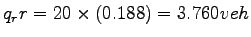
Step 1. Compute the arrival rate throughout the cycle, q:
q = 675/3600 = 0.188 veh/s
Step 2. Compute the net departure rate (saturation flow rate -
arrival rate):
(s - q) =1800/3600- 0.188 = 0.312 veh/s
Step 3.Compute the queue at the end of 20 s of effective red time:
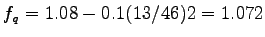
Step 4. Compute the queue calibration factor, : :
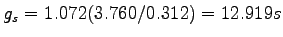
Step 5. Compute the time required to serve the queue,  : :
Step 6. Determine  : :
 = 1.5 and b = 0.6 (for single lane from table in HCM) = 1.5 and b = 0.6 (for single lane from table in HCM)
Step 7. Determine the occupancy time of the detector:
 = 3.6(9.1+ 5.5)/50, vehicle length=5.5m, detector = 1.051 s length=9.1 m,
approach speed=50 kmph = 3.6(9.1+ 5.5)/50, vehicle length=5.5m, detector = 1.051 s length=9.1 m,
approach speed=50 kmph
Step 8. The expected green extension time,  : :
Step 9. Compute the total phase time:
Step 10. Compute the phase time deficiency as the difference
between the trial phase time and the computed phase time:
or 25.469 - 17.0 = 8.469 s.
For next iteration:
Trial green time = 25.469 s.
Cycle length = 50.968 s.
This process is continued through successive iterations until the solutions
converge or the phase deficiency i.e. the error is negligible practically.
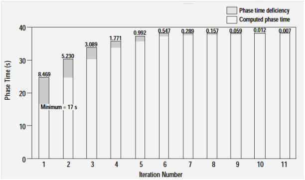
The following figure shows the results of successive iterations for this
problem and the final convergence.
Figure 1:
Calculation of phase time through iterations (HCM)
|
|
The final phase time is 37.710 s giving a cycle length of 75.420 s.
The convergence was considered for threshold of 0.1 difference in successive
cycle times.
|