|
The various types of detectors used for detection of vehicles are as following:
- Inductive loop detectors
- Magnetometer detectors
- Magnetic detectors
- Pressure-sensitive detectors
- Radar detectors
- Sonic detectors
- Microloop detectors etc.
The vast majority of actuated signal installations use inductive loops for
detection purpose.
Now, the type of detection is of greater importance than the specific detection
device(s) used.
There are two types of detection that influence the design and timing of
actuated controllers:
- Passage or Point Detection:- In this type of detection, only
the fact that the detector has been disturbed is noted.
The detector is installed at a point even though the detector unit
itself may involve a short length.
It is the most common form of detection.
- Presence or Area Detection:- In this type of detection, a
significant length (or area) of an approach lane is included in the detection
zone.
Entries and exits of vehicles into and out of the detection zone are
remembered.
Thus, the number of vehicles stored in the detection zone is known.
It is provided by using a long induction loop, or a series of point detectors.
These are generally used in conjunction with volume-density controllers.
Regardless of the controller type, virtually all actuated controllers offer the
same basic functions, although the methodology for implementing them may vary
by type and manufacturer.
For each actuated phase, the following basic features must be set on the
controller:
Each actuated phase has a minimum green time, which serves as the smallest
amount of green time that may be allocated to a phase when it is initiated.
Minimum green times must be set for each phase in an actuated signalization,
including the non-actuated phase of a semi-actuated controller.
The minimum green timing on an actuated phase is based on the type and location
of detectors.
- In case of Point Detectors,
![$\displaystyle G_{min} = t_L + [h \times Integer(d/x)]$](img1.png) |
(1) |
where,
 = minimum green time in second, = minimum green time in second,  = assumed start-up lost time =
4 sec, h = assumed saturation headway = 2 sec, d = distance between detector &
stop line in m and x = assumed distance between stored vehicles = 6 m. = assumed start-up lost time =
4 sec, h = assumed saturation headway = 2 sec, d = distance between detector &
stop line in m and x = assumed distance between stored vehicles = 6 m.
- In case of Area Detectors,
 |
(2) |
where, = start-up lost time (sec) and n = number of vehicles stored in
the detection area.
This time actually serves three different purposes:
- It represents the maximum gap between actuation at a single detector
required to retain the green.
- It is the amount of time added to the green phase when an additional
actuation is received within the unit extension, U.
- It must be of sufficient length to allow a vehicle to travel from the
detector to the STOP line.
In terms of signal operation, it serves as both the minimum allowable gap to
retain a green signal and as the amount of green time added when an additional
actuation is detected within the minimum allowable gap.
The unit extension is selected with two criteria in mind:
- The unit extension should be long enough such that a subsequent vehicle
operating in dense traffic at a safe headway will be able to retain a green
signal (assuming the maximum green has not yet been reached).
- The unit extension should not be so long that straggling vehicles may
retain the green or that excessive time is added to the green (beyond what one
vehicle reasonably requires to cross the STOP line on green).
The Traffic Detector Handbook recommends that a unit extension of 3.0 s be used
where approach speeds are equal to or less than 30 mile per hour, and that 3.5
s be used at higher approach speeds.
For all types of controllers, however, the unit extension must be equal to or
more than the passage time.
It allows a vehicle to travel from the detector to the stop line.
It is analogous with 'Unit Extension'.
 |
(3) |
where, P = passage time, sec, d = distance from detector to stop line, meter
and S = approach speed of vehicles, m/s.
Each phase has a maximum green time that limits the length of a green phase,
even if there are continued actuation that would normally retain the green.
The maximum green time begins when there is a call (or detector
actuation) on a competing phase.
The estimation can be done by any of the following methods:
- By trial signal timing as if the signals were pre-timed
![$\displaystyle C_i = \frac{L}{[1-VC/(1615(PHF)(v/c))]}$](img6.png) |
(4) |
where,  = Initial cycle length, sec, L = Total lost time, sec and = Initial cycle length, sec, L = Total lost time, sec and  =
Sum of critical lane volumes, veh/hr.
Knowing the initial cycle length, green times are then determined as: =
Sum of critical lane volumes, veh/hr.
Knowing the initial cycle length, green times are then determined as:
 |
(5) |
where  = effective green time for Phase i, sec and = effective green time for Phase i, sec and  = critical
lane volume for Phase i, veh/hr.
The effective green times thus obtained are then multiplied by 1.25 or 1.50 to
determine the maximum green time. = critical
lane volume for Phase i, veh/hr.
The effective green times thus obtained are then multiplied by 1.25 or 1.50 to
determine the maximum green time.
- By Green-Time Estimation (HCM) Model:
Traffic-actuated controllers do not recognize specified cycle lengths.
Instead they determine, by a mechanical analogy, the required green time given
the length of the previous red period and the arrival rate.
They accomplish this by holding the right-of-way until the accumulated queue
has been served.
The basic principle underlying all signal timing analysis is the queue
accumulation polygon (QAP), which plots the number of vehicles queued at the
stop line over the duration of the cycle.
The QAP for a simple protected movement is illustrated in the
Fig. 1.
Figure 1:
Queue accumulation polygon illustrating two methods of green time
computation
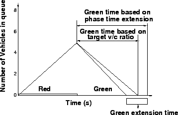 |
From Fig. 1, it's clear that queue accumulation takes
place on the left side of the triangle (i.e., effective red) and the discharge
takes place on the right side of the triangle (i.e., effective green).
There are two methods of determining the required green time given the length
of the previous red time.
The first employs a target v/c approach.
Under this approach, the green-time requirement is determined by the slope of
the line representing the target v/c of 0.9.
If the phase ends when the queue has dissipated under these conditions, the
target v/c will be achieved.
The second method recognizes the way a traffic-actuated controller really
works.
It does not deal explicitly with v/c ratios; in fact, it has no way of
determining the v/c ratio.
Instead it terminates each phase when a gap of a particular length is
encountered at the detector.
Good practice dictates that the gap threshold must be longer than the
gap that would be encountered when the queue is being served.
Assuming that gaps large enough to terminate the phase can only occur after the
queue service interval (based on v/c = 1.0), the average green time may be
estimated as the sum of the queue service time and the phase extension time.
Therefore, average green time = Queue Service Time + Phase Extension Time.
Now,
 |
(6) |
where,  = red arrival rate (veh/s), = red arrival rate (veh/s),  = green arrival rate (veh/s), r
= effective red time (s), s = saturation flow rate (veh/s) and = green arrival rate (veh/s), r
= effective red time (s), s = saturation flow rate (veh/s) and  =
calibration factor = 1.08 - 0.1 =
calibration factor = 1.08 - 0.1
![$\displaystyle \mathrm{Green~extension~time(g_e)} = [exp(\lambda(u+t-\Delta))/\Phi q] -
(1/\lambda)$](img18.png) |
(7) |
where, q = vehicle arrival rate throughout cycle (veh/s), u = unit extension
time setting (s), t = time during which detector is occupied by a passing
vehicle(s) =
![$ [3.6(L_d+L_v)]/S_A$](img19.png) , ,  = Vehicle length, assumed to be 5.5 m, = Vehicle length, assumed to be 5.5 m,
 = Detector length (m), = Detector length (m),  = Vehicle approach speed (kmph), = Vehicle approach speed (kmph),  =
minimum arrival (intra-bunch) headway (s), =
minimum arrival (intra-bunch) headway (s),  = a parameter (veh/s) = = a parameter (veh/s) =
 , ,  = proportion of free (unbunched) vehicles in
traffic stream = = proportion of free (unbunched) vehicles in
traffic stream =
 and b = bunching factor. and b = bunching factor.
This green-time estimation model is not difficult to implement, but it does not
lead directly to the determination of an average cycle length or green time
because the green time required for each phase is dependent on the green time
required by the other phases.
Thus, a circular dependency is established that requires an iterative process
to solve.
With each iteration, the green time required by each phase, given the green
times required by the other phases, can be determined.
The logical starting point for the iterative process involves the minimum times
specified for each phase.
If these times turn out to be adequate for all phases, the cycle length will
simply be the sum of the minimum phase times for the critical phases.
If a particular phase demands more than its minimum time, more time should be
given to that phase.
Thus, a longer red time must be imposed on all of the other phases.
This, in turn, will increase the green time required for the subject phase.
Table 1:
Recommended Parameter Values
| Case |
 |
b |
| Single Lane |
1.5 |
0.6 |
| Multi-lane |
|
|
| 2 lanes |
0.5 |
0.5 |
| 3 lanes |
0.5 |
0.8 |
Each actuated phase has a recall switch.
The recall switches determine what happens to the signal when there is no
demand.
Normally, one recall switch is placed in the on position, while all
others are turned off.
In this case, when there is no demand present, the green returns to the phase
with its recall switch on.
If no recall switch is in the on position, the green remains on the
phase that had the last "call."demand exists, one phase continues to move to the next at the expiration of the
minimum green.
Yellow and all-red intervals provide for safe transition from green to
red.
They are fixed times and are not subject to variation, even in an actuated
controller.
They are found in the same manner as for pre-timed signals.
![$\displaystyle y = t + [S_{85} / (2a+19.6g)]$](img29.png) |
(8) |
 |
(9) |
where, y = yellow time, sec, ar = all red interval, sec,  = 85th
percentile speed, m/s, = 85th
percentile speed, m/s,  = 15th percentile speed, m/s, t = reaction time
of the driver = 1 sec (standard), a = deceleration rate = 3 m/ = 15th percentile speed, m/s, t = reaction time
of the driver = 1 sec (standard), a = deceleration rate = 3 m/ (standard),
g = grade of approach in decimal, w = width of street being crossed, m and l =
length of a vehicle, m. (standard),
g = grade of approach in decimal, w = width of street being crossed, m and l =
length of a vehicle, m.
|
|