| |
| | |
|
The bandwidth concept is very popular in traffic engineering practice, because
- the windows of green (through which platoons of vehicles can move) are
easy visual images for both working professionals and public presentations
- good solutions can often be obtained manually, by trial and error.
The efficiency of a bandwidth (measured in seconds) is defined as the ratio of
the bandwidth to the cycle length, expressed as a percentage:
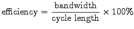 |
(1) |
An efficiency of 40% to 50% is considered good.
The bandwidth is limited by the minimum green in the direction of interest.
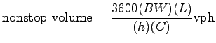
Figure 1:
Bandwidths on a time space diagram
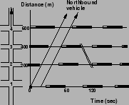 |
Fig. 1 illustrates the bandwidths for one signal-timing plan.
The northbound efficiency can be estimated as
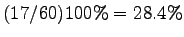 .
There is no bandwidth through the south-bound.
The system is badly in need of re-timing at least on the basis of the bandwidth
objective.
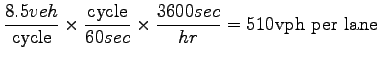
In terms of vehicles that can be put through this system without stopping, note
that the northbound bandwidth can carry .
There is no bandwidth through the south-bound.
The system is badly in need of re-timing at least on the basis of the bandwidth
objective.
In terms of vehicles that can be put through this system without stopping, note
that the northbound bandwidth can carry
 vehicles per lane per
cycle in a nonstop path through the defined system.
The northbound direction can handle
very efficiently if they are organized into 8-vehicle platoons when they arrive
at this system.
If the per lane demand volume is less than vehicles per lane per
cycle in a nonstop path through the defined system.
The northbound direction can handle
very efficiently if they are organized into 8-vehicle platoons when they arrive
at this system.
If the per lane demand volume is less than  and if the flows are so
organized, the system will operate well in the northbound direction, even
though better timing plans might be obtained.
The computation can be formalized into an equation as follows: and if the flows are so
organized, the system will operate well in the northbound direction, even
though better timing plans might be obtained.
The computation can be formalized into an equation as follows:
 |
(2) |
where:  = measured or computed bandwidth, sec, = measured or computed bandwidth, sec,  = number of through lanes
in indicated direction, = number of through lanes
in indicated direction,  = headway in moving platoon, sec/veh,and = headway in moving platoon, sec/veh,and  =cycle length.
The engineer usually wishes to design for maximum bandwidth in one direction,
subject to some relation between the bandwidths in the two directions.
There are both trial-and-error and somewhat elaborate manual techniques for
establishing maximum bandwidths.
Refer to Fig. 2, which shows four signals and decent progressions
in both the directions.
For purpose of illustration, assume it is given that a signal with 50:50 split
may be located midway between Intersections 2 and 3.
The possible effect as it appears in Fig. 3 is that there is no
way to include this signal without destroying one or the other through band, or
cutting both in half.
The offsets must be moved around until a more satisfactory timing plan
develops.
A change in cycle length may even be required.
The changes in offset may be explored by:
=cycle length.
The engineer usually wishes to design for maximum bandwidth in one direction,
subject to some relation between the bandwidths in the two directions.
There are both trial-and-error and somewhat elaborate manual techniques for
establishing maximum bandwidths.
Refer to Fig. 2, which shows four signals and decent progressions
in both the directions.
For purpose of illustration, assume it is given that a signal with 50:50 split
may be located midway between Intersections 2 and 3.
The possible effect as it appears in Fig. 3 is that there is no
way to include this signal without destroying one or the other through band, or
cutting both in half.
The offsets must be moved around until a more satisfactory timing plan
develops.
A change in cycle length may even be required.
The changes in offset may be explored by:
- copying the time-space diagram of Fig. 3
- cutting the copy horizontally into strips, one strip per intersection
- placing a guideline over the strips, so as to indicate the speed of the
platoon(s) by the slope of the guideline
- sliding the strips relative to each other, until some improved offset
pattern is identified
Figure 2:
Case study:Four intersections with good progressions
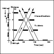 |
Figure 3:
Effect of inserting a new signal into system
 |
There is no need to produce new strips for each cycle length considered: all
times can be made relative to an arbitrary cycle length `C.
The only change necessary is to change the slope(s) of the guidelines
representing the vehicle speeds.
The northbound vehicle takes
 to travel from intersection 4
to intersection 2.
If the cycle length to travel from intersection 4
to intersection 2.
If the cycle length
 , the vehicle would have arrived at
intersection 2 at , the vehicle would have arrived at
intersection 2 at  , or one half of the cycle length.
To obtain a good solution through trial-and-error attempt, the following should
be kept in consideration: , or one half of the cycle length.
To obtain a good solution through trial-and-error attempt, the following should
be kept in consideration:
- If the green initiation at Intersection 1 comes earlier, the southbound
platoon is released sooner and gets stopped or disrupted at intersection 2.
- Likewise, intersection 2 cannot be northbound without harming the
southbound.
- Nor can intersection 3 help the southbound without harming the
northbound.
An elegant mathematical formulation requiring two hours of computation on a
supercomputer is some-what irrelevant in most engineering offices.
The determination of good progressions on an arterial must be viewed in this
context:only 25 years ago, hand held calculators did not exist; 20 years ago,
calculators had only the most basic functions.
15 years ago, personal computers were at best a new concept.
Previously, engineers used slide rules.
Optimization of progressions could not depend on mathematical formulations
simply because even one set of computations could take days with t he tools
available.
Accordingly,graphical methods were developed.
The first optimization programs that took queues and other details into account
began to appear, leading to later developments that produced the
signal-optimization programs in common use in late 1980s.
As computers became more accessible and less expensive, the move to computer
solutions accelerated in the 1970s.
New work on the maximum-bandwidth solution followed with greater computational
power encouraging the new formulations.
|
|
| | |
|
|
|