| |
| | |
|
A basic freeway segment can be characterized by three performance measures:
density in terms of passenger cars per kilometer per lane, speed in terms of
mean passenger-car speed, and volume-to-capacity (v/c) ratio.
Each of these measures is an indication of how well traffic flow is being
accommodated by the freeway.
The measure used to provide an estimate of level of service is density.
The three measures of speed, density, and flow or volume are interrelated.
If values for two of these measures are known, the third can be computed.
Level of service of an existing freeway is determined considering it as a stretch of basic freeway segment.
It means that we have to take all the base conditions decided for basic freeway segment as a standard or initial input.
The following steps are followed to determine the level of service of a freeway.
- The very first step of methodology is to collect all the input data like geometric data, measured FFS or BFFS, volume.
- volume adjustment: The hourly volume is converted into flow rate of passenger cars i.e pc/hr/ln.
- Computation of FFS: If BFFS is the input, then for getting the value of FFS ,we have to adjust the BFFS for the lane width,number of lanes,interchange density and lateral clearance.
- computation of S(average passenger car speed): S is calculated from the FFS. If FFS is measured directly in field, then FFS can be taken as S.
- Speed-flow curve is designed and speed is determined using this curve.
- Density is determined from the flow rate and speed taken from the speed-flow curve.
- Based on the density, the corresponding level of service(LOS) can be determined .
The steps involved in calculation of LOS are-
- Calculation of flow rate (
 ) )
- Calculation of average passenger car (
 ) )
- Calculation of density (
 ) and determining LOS ) and determining LOS
The hourly flow rate must reflect the influence of heavy vehicles, the temporal
variation of traffic flow over an hour, and the characteristics of the driver
population.
These effects are reflected by adjusting hourly volumes or estimates, typically
reported in vehicles per hour (veh/h), to arrive at an equivalent passenger-car
flow rate in passenger cars per hour (pc/h).
The equivalent passenger-car flow rate is calculated using the heavy-vehicle and
peak-hour adjustment factors and is reported on a per lane basis (pc/h/ln).
The flow rate can be given as-
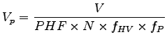 |
(1) |
where,  = hourly volume, = hourly volume,  = peak hour factor (0.80-0.95), = peak hour factor (0.80-0.95),  = no. of lanes, = no. of lanes,  = heavy vehicle adjustment factor, = heavy vehicle adjustment factor,  = driver population factor
The peak-hour factor (PHF) represents the variation in traffic flow within an
hour.
Observations of traffic flow consistently indicate that the flow rates found in
the peak 15-min period within an hour are not sustained throughout the entire hour. = driver population factor
The peak-hour factor (PHF) represents the variation in traffic flow within an
hour.
Observations of traffic flow consistently indicate that the flow rates found in
the peak 15-min period within an hour are not sustained throughout the entire hour.
 |
(2) |
Where, = hourly volume in veh/hr for hour of analysis,  = Maximum 15-min flow rate within peak hour, = Maximum 15-min flow rate within peak hour,  = number of 15-min period per hour. = number of 15-min period per hour.
On freeways, typical PHFs range from 0.80 to 0.95.
Lower PHFs are characteristic of rural freeways or off-peak conditions.
Higher factors are typical of urban and suburban peak-hour conditions.
Field data should be used, if possible, to develop PHFs representative of local
conditions.
Freeway traffic volumes that include a mix of vehicle types must be adjusted to
an equivalent flow rate expressed in passenger cars per hour per lane.
This adjustment is made using the factor .
Once the values of  and and  are found, the adjustment factor, ,
is determined by using equation given below - are found, the adjustment factor, ,
is determined by using equation given below -
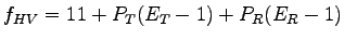 |
(3) |
where, , = passenger car equivalents for truck buses and recreational
vehicles (RV's) in traffic stream respectively,  , ,  = proportion of truck/buses and recreational vehicles in traffic
stream.
Adjustments for heavy vehicles in the traffic stream apply for three vehicle
types: trucks, buses, and RVs.
There is no evidence to indicate distinct differences in performance between
trucks and buses on freeways, and therefore trucks and buses are treated
identically.
The factor is found using a two-step process.
First, the passenger-car equivalent for each truck/bus and RV is found for the
traffic and roadway conditions under study.
These equivalence values, and , represent the number of passenger
cars that would use the same amount of freeway capacity as one truck/bus or RV,
respectively, under prevailing roadway and traffic conditions.
Second, using the values of and and the proportion of each type of
vehicle in the traffic stream ( and ), the adjustment factor
is computed.
Under base conditions, the traffic stream is assumed to consist of regular weekday drivers and commuters.Such drivers have a high familiarity with the roadway and generally maneuver and respond to the maneuvers of other drivers in a safe and predictable fashion.
But weekend drivers or recreational drivers are a problem. Such drivers can cause a significant reduction in roadway capacity relative to the base condition of having only familiar drivers.
To account for the composition of the driver population, the fp adjustment
factor is used and its recommended range is 0.85 – 1.00. = proportion of truck/buses and recreational vehicles in traffic
stream.
Adjustments for heavy vehicles in the traffic stream apply for three vehicle
types: trucks, buses, and RVs.
There is no evidence to indicate distinct differences in performance between
trucks and buses on freeways, and therefore trucks and buses are treated
identically.
The factor is found using a two-step process.
First, the passenger-car equivalent for each truck/bus and RV is found for the
traffic and roadway conditions under study.
These equivalence values, and , represent the number of passenger
cars that would use the same amount of freeway capacity as one truck/bus or RV,
respectively, under prevailing roadway and traffic conditions.
Second, using the values of and and the proportion of each type of
vehicle in the traffic stream ( and ), the adjustment factor
is computed.
Under base conditions, the traffic stream is assumed to consist of regular weekday drivers and commuters.Such drivers have a high familiarity with the roadway and generally maneuver and respond to the maneuvers of other drivers in a safe and predictable fashion.
But weekend drivers or recreational drivers are a problem. Such drivers can cause a significant reduction in roadway capacity relative to the base condition of having only familiar drivers.
To account for the composition of the driver population, the fp adjustment
factor is used and its recommended range is 0.85 – 1.00.
|
|
| | |
|
|
|