Module 4 : Macroscopic And Mesoscopic Traffic Flow Modeling

Lecture 19 : Traffic Progression Models

1

2

3

4

5

6

7

8

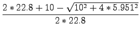
	Numerical Example 1 In a case study, the average travel time for a particular stretch was found out to be 22.8 seconds, standard deviation is 5.951 and model time step duration is 10 sec. Find out the Robertson's model parameters and also the flow at downstream at different time steps where the upstream flows are as given as: $q_{10~sec} = 20, q_{20~sec} = 10, q_{30~sec} = 15, q_{40~sec} = 18, q_{50~sec} = 14, q_{60~sec} = 12$. 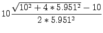Solution Given, The model time step duration n=10sec, average travel time ($T_a$)=22.8sec, standard deviation ($\sigma$)=5.951. From equations above. $$\beta_n = \frac{2T_a+n-\sqrt{n^2+4\sigma^2}}{2T_a}$$ $$= \frac{2*22.8+10-\sqrt{10^2+4*5.951^2}}{2*22.8}$$ $$= 0.878$$ $$\alpha_n = \frac{1-\beta_{n}}{\beta_{n}}$$ $$= \frac{1-0.878}{0.878}$$ $$= 0.139$$ $$F_{n} = n\frac{\sqrt{n^2+4\sigma^2}-n}{2\sigma^2}$$ $$= 10\frac{\sqrt{10^2+4*5.951^2}-10}{2*5.951^2}$$ $$= 0.783$$ Upstream Flows: Since the modelling time step duration is given as n=10 sec, the given upstream flows can be written as follows: $$q_{10~sec} = q_1$$ $$q_{20~sec} = q_2$$ $$q_{30~sec} = q_3$$ On similar lines , $q_4$, $q_5$, $q_6$ can be written. Downstream Flows: On the downstream, at 10 sec the flow will be zero since the modelling step duration is 10 sec. 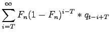Hence the downstream flows can be written as follows. $$q^{d}_{20~sec} = q^{d}_1$$ $$q^{d}_{30~sec} = q^{d}_2$$ $$q^{d}_{40~sec} = q^{d}_3$$ Similarly, downstream flows can be written till 80 sec. Note that since n=10 sec, T is taken in units of n. 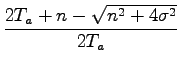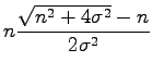The minimum travel time (T) is given as $$T = \beta T_a = 0.878 * 22.8 = 20~sec = 2$$ $$q_t^d = \sum_{i=T}^\infty{F_n(1-F_n)^{i-T}*q_{t-i+T}}$$ $$q_{1}^d = F * (1-F)^{2-2}*q_{1-2+2}$$ $$= F*q_{1}$$ $$= 0.783 * 20 = 15.66 \approx 16~veh$$ $$q_{2}^d = F*(1-F)^{2-2}*q_{2-2+2} + F*(1-F)^{3-2}*q_{2-3+2}$$ $$= F * q_{2} + F * (1-F)^1 * q_{1}$$ $$= 0.783 x 10 + 0.783 * (1-0.783)^1 * 20$$ $$= 7.83 + 3.39 = 11.22 \approx 11~veh$$ $$q_{3}^d = F*(1-F)^{2-2}*q_{3-2+2}+F*(1-F)^{3-2}*q_{3+2}+F*(1-F)^{4-2}*q_{3-4+2}$$ $$= F*q_{3} +F*(1-F)^1*q_{2} + F * (1-F)^2*q_{1}$$ $$= 0.783*15+ 0.783*(1-0.783)^1*10+0.783*(1-0.783)^2*20$$ $$= 11.75 + 1.69 + 0.737 = 14.18 \approx 14~veh$$ Calculating on similar lines, we get $$q_{4}^d(50~sec) = 17~veh$$ $$q_{5}^d(60~sec) = 15~veh$$ $$q_{6}^d(70~sec) = 13~veh$$ $$q_{7}^d(80~sec) = 3~veh$$ The total upstream vehicles in 60 sec is 89. And total downstream vehicles in 80 sec is 89. That is, all 89 vehicles coming from upstream in 6 intervals took 7 intervals to pass the downstream.