The basic Robertson's recursive platoon dispersion model takes the following
mathematical form
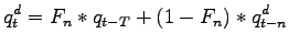 |
(1) |
where,  = arrival flow rate at the downstream signal at time t, = arrival flow rate at the downstream signal at time t,
 = departure flow rate at the upstream signal at time t-T, T = minimum
travel time on the link (measured in terms of unit steps T = = departure flow rate at the upstream signal at time t-T, T = minimum
travel time on the link (measured in terms of unit steps T = ), ),  = average link travel time, n = modeling time step duration,
  is the
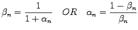
smoothing factor given by: is the
smoothing factor given by:
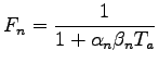 |
(2) |
 = platoon dispersion factor (unit less) = platoon dispersion factor (unit less)
 = travel time factor (unit less)
Equation shows that the arrival flows in each time period at each intersection
are dependent on the departure flows from other intersections.
Note that the Robertson's platoon dispersion equation means that the traffic
flow = travel time factor (unit less)
Equation shows that the arrival flows in each time period at each intersection
are dependent on the departure flows from other intersections.
Note that the Robertson's platoon dispersion equation means that the traffic
flow  , which arrives during a given time step at the downstream end of
a link, is a weighted combination of the arrival pattern at the downstream end
of the link during the previous time step , which arrives during a given time step at the downstream end of
a link, is a weighted combination of the arrival pattern at the downstream end
of the link during the previous time step  and the departure pattern
from the upstream traffic signal T seconds ago . and the departure pattern
from the upstream traffic signal T seconds ago .
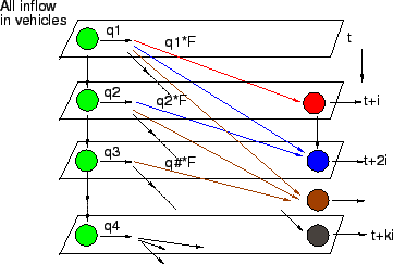
Fig. 1 gives the graphical representation of the model.
It clearly shows that predicated flow rate at any time step is a linear
combination of the original platoon flow rate in the corresponding time step
(with a lag time of t) and the flow rate of the predicted platoon in the step
immediately preceding it.
Since the dispersion model gives the downstream flow at a given time interval,
the model needs to be applied recursively to predict the flow.
Seddon developed a numerical procedure for platoon dispersion.
He rewrote Robertson's equation as,
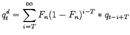 |
(3) |
Figure 1:
Graphical Representation of Robertson's Platoon Dispersion Model
 |
This equation demonstrates that the downstream traffic flow computed using the
Robertson's platoon dispersion model follows a shifted geometric series, which
estimates the contribution of an upstream flow in the
 interval to
the downstream flow in the interval to
the downstream flow in the  interval.
A successful application of Robertson's platoon dispersion model relies on the
appropriate calibration of the model parameters.
Research has shown that the travel-time factor interval.
A successful application of Robertson's platoon dispersion model relies on the
appropriate calibration of the model parameters.
Research has shown that the travel-time factor  is dependent on the
platoon dispersion factor is dependent on the
platoon dispersion factor
 .
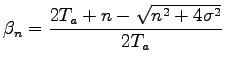
Using the basic properties of the geometric distribution of Equation 1, the
following equations have been derived for calibrating the parameters of the
Robertson platoon dispersion model. .
Using the basic properties of the geometric distribution of Equation 1, the
following equations have been derived for calibrating the parameters of the
Robertson platoon dispersion model.
 |
(4) |
Equation 4 demonstrates that the value of the travel time factor  is
dependent on the value of the platoon dispersion factor is
dependent on the value of the platoon dispersion factor  and thus a
value of 0.8 as assumed by Robertson results in inconsistencies in the
formulation.
Further, the model requires calibration of only one of them and the other
factors can be obtained subsequently. and thus a
value of 0.8 as assumed by Robertson results in inconsistencies in the
formulation.
Further, the model requires calibration of only one of them and the other
factors can be obtained subsequently.
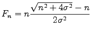
 |
(5) |
where,  is the standard deviation of link travel times and is the
average travel time between upstream and downstream intersections.
Equation demonstrates that travel time factor can be obtained knowing the
average travel time, time step for modeling and standard deviation of the travel
time on the road stretch. is the standard deviation of link travel times and is the
average travel time between upstream and downstream intersections.
Equation demonstrates that travel time factor can be obtained knowing the
average travel time, time step for modeling and standard deviation of the travel
time on the road stretch.
 |
(6) |
Equation 6 further permits the calculation of the smoothing factor directly from
the standard deviation of the link travel time and time step of modeling.
Thus, both and can be mathematically determined as long as the
average link travel time, time step for modeling and its standard deviation are
given.
|