| |
| | |
|
As sequel to his first paper on CTM, Daganzo (1995) published first paper on
CTM applied to network traffic.
In this section application of CTM to network traffic considering merging and
diverging is discussed.
Some basic notations: (The notations used from here on, are adopted from
Ziliaskopoulos (2000))
 = Set of predecessor cells. = Set of predecessor cells.  =
Set of successor cells.
The notations introduced in previous section
are applied to different types of cells, as shown in
Figures 1, 2 & 3.
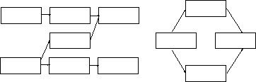
Some valid and invalid representations in a network are shown in
Fig 7 & Fig 6. =
Set of successor cells.
The notations introduced in previous section
are applied to different types of cells, as shown in
Figures 1, 2 & 3.
Some valid and invalid representations in a network are shown in
Fig 7 & Fig 6.
Figure 1:
Source Cell
 |
Figure 2:
Sink Cell
 |
Figure 3:
Ordinary Cell
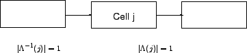 |
Figure 4:
Merging Cell
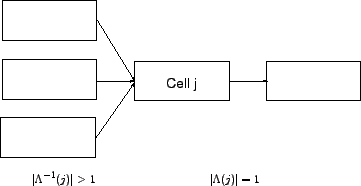 |
Figure 5:
Diverging Cell
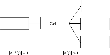 |
Figure 6:
Invalid representations
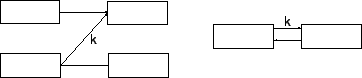 |
Figure 7:
Valid representations
 |
Consider an ordinary link with a beginning cell and ending cell, which gives
the flow between two cells is simplified as explained below.
Figure 8:
Ordinary Link
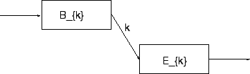 |
![$\displaystyle y_k(t) = min(n_{Bk}(t), min[Q_{Bk}(t), Q_{Ek}(t)], \delta_{Ek}[ NEk(t) -
nEk(t)])$](img11.png) |
(1) |
where,
 . .
 is the inflow to cell Ek in the time interval ( is the inflow to cell Ek in the time interval ( , , ).
Defining the maximum flows that can be sent and received by the cell i in the
interval between to as ).
Defining the maximum flows that can be sent and received by the cell i in the
interval between to as
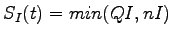 , and , and
![$ R_I(t) = min (Q_I,\delta_I,[N_I- n_I])$](img17.png) .
Therefore, can be written in a more compact form as: .
Therefore, can be written in a more compact form as:
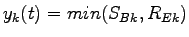 .
This means that the flow on link k should be the maximum that can be sent by
its upstream cell unless prevented to do so by its end cell.
If blocked in this manner, the flow is the maximum allowed by the end cell.
From equations one can see that a simplification is done by splitting
in to .
This means that the flow on link k should be the maximum that can be sent by
its upstream cell unless prevented to do so by its end cell.
If blocked in this manner, the flow is the maximum allowed by the end cell.
From equations one can see that a simplification is done by splitting
in to  and and  terms.
'S' represents sending capacity and 'R' represents receiving capacity.
During time periods when terms.
'S' represents sending capacity and 'R' represents receiving capacity.
During time periods when
 the flow on link k is dictated by
upstream traffic conditions-as would be predicted from the forward moving
characteristics of the Hydrodynamic model.
Conversely, when the flow on link k is dictated by
upstream traffic conditions-as would be predicted from the forward moving
characteristics of the Hydrodynamic model.
Conversely, when
 , flow is dictated by downstream conditions
and backward moving characteristics. , flow is dictated by downstream conditions
and backward moving characteristics.
|
|
| | |
|
|
|