| |
| | |
|
The cell transmission model simulates traffic conditions by proposing to
simulate the system with a time-scan strategy where current
conditions are updated with every tick of a clock.
The road section under consideration is divided into homogeneous sections
called cells, numbered from  = 1 to I.
The lengths of the sections are set equal to the distances travelled in
light traffic by a typical vehicle in one clock tick.
Under light traffic condition, all the vehicles in a cell can be
assumed to advance to the next with each clock tick. i.e, = 1 to I.
The lengths of the sections are set equal to the distances travelled in
light traffic by a typical vehicle in one clock tick.
Under light traffic condition, all the vehicles in a cell can be
assumed to advance to the next with each clock tick. i.e,
 |
(1) |
where,
 is the number of vehicles in cell at time is the number of vehicles in cell at time  .
However, equation 1 is not reasonable when flow exceeds the capacity.
Hence a more robust set of flow advancement equations are presented in a later section.
First, two constants associated with each cell are defined, they are:
(i) .
However, equation 1 is not reasonable when flow exceeds the capacity.
Hence a more robust set of flow advancement equations are presented in a later section.
First, two constants associated with each cell are defined, they are:
(i)  which is the maximum number of vehicles that can
be present in cell at time , it is the product of the cell's
length and its jam density.
(ii) which is the maximum number of vehicles that can
be present in cell at time , it is the product of the cell's
length and its jam density.
(ii)  is the maximum number of vehicles that can
flow into cell when the clock advances from to is the maximum number of vehicles that can
flow into cell when the clock advances from to  (time
interval ), it is the minimum of the capacity of cells from (time
interval ), it is the minimum of the capacity of cells from
 and .
It is called the capacity of cell .
It represents the maximum flow that can be transferred from to
.
We allow these constants to vary with time to be able to model transient
traffic incidents.
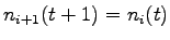
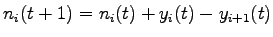
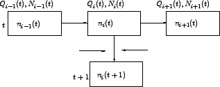
Now the flow advancement equation can be written as, the cell occupancy at time
equals its occupancy at time t, plus the inflow and minus the outflow;
i.e., and .
It is called the capacity of cell .
It represents the maximum flow that can be transferred from to
.
We allow these constants to vary with time to be able to model transient
traffic incidents.
Now the flow advancement equation can be written as, the cell occupancy at time
equals its occupancy at time t, plus the inflow and minus the outflow;
i.e.,
 |
(2) |
where,  is the cell occupancy at time , the cell
occupancy at time , is the cell occupancy at time , the cell
occupancy at time ,  is the inflow at time , is the inflow at time ,
 is the
outflow at time .
The flows are related to the current conditions at time as
indicated below: is the
outflow at time .
The flows are related to the current conditions at time as
indicated below:
![$\displaystyle y_i(t) = min~[n_{i-1}(t), Q_i(t), N_i(t) - n_i(t)]$](img13.png) |
(3) |
where,
 : is the number of vehicles in cell at time
, : is the number of vehicles in cell at time
,  : is the capacity flow into for time interval ,
- : is the amount of empty space in cell at time
. : is the capacity flow into for time interval ,
- : is the amount of empty space in cell at time
.
Figure 1:
Flow advancement
 |
Boundary conditions are specified by means of input and output cells.
The output cell, a sink for all exiting traffic, should have infinite
size (
 ) and a suitable, possibly time-varying,
capacity.
Input flows can be modeled by a cell pair.
A source cell numbered 00 with an infinite number of
vehicles ( ) and a suitable, possibly time-varying,
capacity.
Input flows can be modeled by a cell pair.
A source cell numbered 00 with an infinite number of
vehicles (
 ) that discharges into an empty gate
cell 00 of infinite size, ) that discharges into an empty gate
cell 00 of infinite size,
 .
The inflow capacity .
The inflow capacity  of the gate cell is set equal to the
desired link input flow for time interval . of the gate cell is set equal to the
desired link input flow for time interval .
|
|
| | |
|
|
|