| |
| | |
|
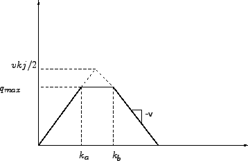
Consider equations ![[*]](file:/usr/local/share/lib/latex2html/icons/crossref.png) & , they are discrete approximations
to the hydrodynamic model with a density- flow (k-q) relationship in the
shape of an isoscaled trapezoid, as in Fig.1.
This relationship can be expressed as: & , they are discrete approximations
to the hydrodynamic model with a density- flow (k-q) relationship in the
shape of an isoscaled trapezoid, as in Fig.1.
This relationship can be expressed as:
![$\displaystyle q = min~[v_k, q_{max}, v(k_j - k)], for~0 \leq k \leq k_j,$](img1.png) |
(1) |
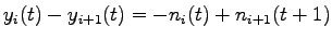
Flow conservation is given by,
 |
(2) |
To demonstrate the equivalence of the discrete and continuous
approaches, the clock tick set to be equal to
 and choose
the unit of distance such that and choose
the unit of distance such that
 = 1.
Then the cell length is 1, = 1.
Then the cell length is 1,  is also 1, and the following
equivalences hold: is also 1, and the following
equivalences hold:
 , ,
 , ,
 , and , and
 with these conventions, it can be easily seen that the
equations 1 & are equivalent.
Equation 3 can be equivalently written as: with these conventions, it can be easily seen that the
equations 1 & are equivalent.
Equation 3 can be equivalently written as:
 |
(3) |
This represents change in flow over space equal to change in occupancy over
time.
Rearranging terms of equation we can arrive at equation ,
which is the same as the basic flow advancement equation of the cell
transmission model.
Figure 1:
Flow-density relationship for the basic cell-transmission model
 |
|
|
| | |
|
|
|