Consider a 1.25 km homogeneous road with speed
 , jam density , jam density
 and and
 .
Initially traffic is flowing undisturbed at 80% of capacity: .
Initially traffic is flowing undisturbed at 80% of capacity:
 .
Then, a partial lane blockage lasting 2 min occurs on .
Then, a partial lane blockage lasting 2 min occurs on  of the
distance from the end of the road.
The blockage effectively restricts flow to 20% of the maximum.
Clearly, a queue is going to build and dissipate behind the restriction.
After 2 minutes, the flow in cell 3 is maximum possible flow.
Predict the evolution of the traffic.
Take one clock tick as 30 seconds.
The main purpose of cell transmission model is to simulate the real traffic
conditions for a defined stretch of road.
The speed and cell length is kept constant and also the cell lengths in cell
transmission model.
The solution has been divided into 4 steps as follows: of the
distance from the end of the road.
The blockage effectively restricts flow to 20% of the maximum.
Clearly, a queue is going to build and dissipate behind the restriction.
After 2 minutes, the flow in cell 3 is maximum possible flow.
Predict the evolution of the traffic.
Take one clock tick as 30 seconds.
The main purpose of cell transmission model is to simulate the real traffic
conditions for a defined stretch of road.
The speed and cell length is kept constant and also the cell lengths in cell
transmission model.
The solution has been divided into 4 steps as follows:
Step 1: Determination of cell length and number of cells
Given clock tick,
 of an hour.
So, cell length = distance travelled by vehicle in one clock tick = of an hour.
So, cell length = distance travelled by vehicle in one clock tick =
 .
Road stretch given = .
Road stretch given =  .
Therefore, no of cells = .
Therefore, no of cells =
 = = 
Step 2: Determination of constants (N & Q)
N = maximum number of vehicles that can be at time t in cell i,
= cell length x jam density,
= 180 x (5/12) = 75 vehicles,
Q = maximum number of vehicles that can flow into cell I from time t to t+1,
= 3000 x (1/120) = 25 vehicles.
Now, to simulate the traffic conditions for some time interval, our main aim is
to find the occupancies of the 3 cells (as calculated above) with the
progression of clock tick.
This is easily showed by creating a table.
First of all, the initial values in the tables are filled up.
Step 3: Determination of cell capacity in terms of number
of vehicles for various traffic flows.
For 20% of the maximum =
 .
For 80% of the maximum = .
For 80% of the maximum =
 . .
Step 4: Initialization of the table
The table has been prepared with source cell as a large capacity value and a
gate is there which connects and regulates the flow of vehicles from source to
cell 1 as per the capacity of the cell for a particular interval.
The cell constants ( and and  ) for the 3 cells are shown in the table. Note
that the sink can accommodate maximum number of vehicles whichever the cell 3
generates.
Q3 is the capacity in terms of number of vehicles of cell 3 .
The value from H5 to H7 (i.e 5) corresponds to the 2min time interval with 4
clock ticks when the lane was blocked so the capacity reduced to 20% of the
maximum (i.e. 600 ) for the 3 cells are shown in the table. Note
that the sink can accommodate maximum number of vehicles whichever the cell 3
generates.
Q3 is the capacity in terms of number of vehicles of cell 3 .
The value from H5 to H7 (i.e 5) corresponds to the 2min time interval with 4
clock ticks when the lane was blocked so the capacity reduced to 20% of the
maximum (i.e. 600  (1/120) vehicles).
After the 2 min time interval is passed vehicles flows with full capacity in
cell 3.
So the value is 25 (i.e 3000 (1/120) vehicles). (1/120) vehicles).
After the 2 min time interval is passed vehicles flows with full capacity in
cell 3.
So the value is 25 (i.e 3000 (1/120) vehicles).
Table 1:
Entries at the start of the simulation.
| |
Source(00) |
Gate(0) |
Cell1 |
Cell2 |
Cell3 |
Cell4 |
|
| Q |
|
20 |
25 |
25 |
|
25 |
|
| N |
|
999 |
75 |
75 |
75 |
999 |
|
| Time |
|
|
|
|
|
|
Q3 |
| 1 |
999 |
20 |
20 |
20 |
20 |
|
5 |
| 2 |
999 |
20 |
|
|
|
|
5 |
| 3 |
999 |
20 |
|
|
|
|
5 |
| 4 |
999 |
20 |
|
|
|
|
5 |
| 5 |
999 |
20 |
|
|
|
|
25 |
| 6 |
999 |
20 |
|
|
|
|
25 |
| 7 |
999 |
20 |
|
|
|
|
25 |
| 8 |
999 |
20 |
|
|
|
|
25 |
| 9 |
999 |
20 |
|
|
|
|
25 |
| 10 |
999 |
20 |
|
|
|
|
25 |
| 11 |
999 |
20 |
|
|
|
|
25 |
| 12 |
999 |
20 |
|
|
|
|
25 |
| 13 |
999 |
20 |
|
|
|
|
25 |
| 14 |
999 |
20 |
|
|
|
|
25 |
| 15 |
999 |
20 |
|
|
|
|
25 |
| 16 |
999 |
20 |
|
|
|
|
25 |
| 17 |
999 |
20 |
|
|
|
|
25 |
| 18 |
999 |
20 |
|
|
|
|
25 |
|
Step 5: Computation of Occupancies
Simulation need not be started in any specific order, it can be started from
any cell in the row corresponding to the current clock tick.
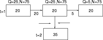
Now, consider cell circled (cell 2 at time 2) in the final table.
Its entry depends on the cells marked with rectangles.
By flow conservation law:
Occupancy = Storage + Inflow - Outflow.
Note that the Storage is the occupancy of the same cell from the preceding
clock tick.
Also outflow of one cell is equal to the inflow of the just
succeeding cell.
Here,
Storage = 20.
For inflow use equation ![[*]](file:/usr/local/share/lib/latex2html/icons/crossref.png) Inflow= min [20,min(25,25),(75-20)]= 20.
Outflow= min [20,min(25,5),(75-20)]= 5.
Occupancy= 20+20-5=35.
Inflow= min [20,min(25,25),(75-20)]= 20.
Outflow= min [20,min(25,5),(75-20)]= 5.
Occupancy= 20+20-5=35.
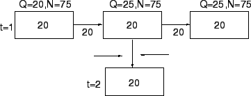
Now,
For cell 1 at time 2,
Inflow= min [20,min(25,25),(75-20)]= 20,
Outflow= min [20,min(25,25),(75-20)]= 20,
Occupancy= 20+20-20=20.
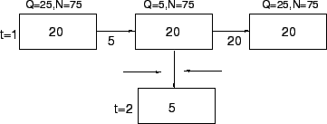
Now,
For cell 3 at time 2,
Inflow= min [20, min (25,5),(75-20)]= 5.
Outflow= 20 (:.sink cell takes all the vehicles in previous cell)
Occupancy= 20+5-20=5.
Similarly, rest of the entries can be filled and the final result is shown in
Table below.
Table 2:
Final entries simulating the traffic
| |
Source(00) |
Gate(0) |
Cell 1 |
Cell 2 |
Cell 3 |
Cell 4 |
|
| Q |
|
20 |
25 |
25 |
|
25 |
|
| N |
|
999 |
75 |
75 |
75 |
999 |
|
| Time |
|
|
|
|
|
|
Q3 |
| 1 |
999 |
20 |
20 |
20 |
20 |
|
5 |
| 2 |
999 |
20 |
20 |
35 |
5 |
|
5 |
| 3 |
999 |
20 |
20 |
50 |
5 |
|
5 |
| 4 |
999 |
20 |
20 |
65 |
5 |
|
5 |
| 5 |
999 |
20 |
30 |
70 |
5 |
|
25 |
| 6 |
999 |
20 |
45 |
50 |
25 |
|
25 |
| 7 |
999 |
20 |
40 |
50 |
25 |
|
25 |
| 8 |
999 |
20 |
35 |
50 |
25 |
|
25 |
| 9 |
999 |
20 |
30 |
50 |
25 |
|
25 |
| 10 |
999 |
20 |
25 |
50 |
25 |
|
25 |
| 11 |
999 |
20 |
20 |
50 |
25 |
|
25 |
| 12 |
999 |
20 |
20 |
45 |
25 |
|
25 |
| 13 |
999 |
20 |
20 |
40 |
25 |
|
25 |
| 14 |
999 |
20 |
20 |
35 |
25 |
|
25 |
| 15 |
999 |
20 |
20 |
30 |
25 |
|
25 |
| 16 |
999 |
20 |
20 |
25 |
25 |
|
25 |
| 17 |
999 |
20 |
20 |
20 |
25 |
|
25 |
| 18 |
999 |
20 |
20 |
20 |
20 |
|
25 |
|
From the table it can be seen that the occupancy i.e. the number of vehicles on
cell 1 and 2 increases and then decreases simulating the effect of lane
blockage in cell 3 on cell 1 and cell 2.
The lane blockage lasts 2 minutes in this problem, after that there is no
congestion taken into account.
So as the time passes by, the occupancy in cell 1 and cell 2 also gets reduced.
|