| |
| | |
|
The relation between time mean speed and space mean speed can be derived as
below.
Consider a stream of vehicles with a set of sub-stream flow  , ,  , ... , ...
 , ... , ... having speed having speed  , , , ... , ... , ... , ... .
The fundamental relation between flow( .
The fundamental relation between flow( ), density( ), density( ) and mean speed ) and mean speed  is,
is,
 |
(1) |
Therefore for any sub-stream , the following relationship will be valid.
 |
(2) |
The summation of all sub-stream flows will give the total flow :
 |
(3) |
Similarly the summation of all sub-stream density will give the total density
.
 |
(4) |
Let  denote the proportion of sub-stream density denote the proportion of sub-stream density  to the total density
, to the total density
,
 |
(5) |
Space mean speed averages the speed over space.
Therefore, if vehicles has speed, then space mean speed is given
by,
 |
(6) |
Time mean speed averages the speed over time. Therefore,
 |
(7) |
Substituting 2,  can be written as, can be written as,
 |
(8) |
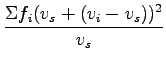
Rewriting the above equation and substituting 5, and then
substituting 1, we get,
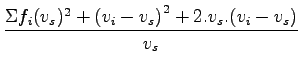
By adding and subtracting and doing algebraic manipulations, can be
written as,
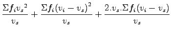
The third term of the equation will be zero because
 will
be zero, since is the mean speed of .
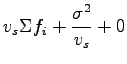
The numerator of the second term gives the standard deviation of . will
be zero, since is the mean speed of .
The numerator of the second term gives the standard deviation of .
 by definition is 1.Therefore, by definition is 1.Therefore,
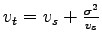
Hence, time mean speed is space mean speed plus standard deviation of the spot
speed divided by the space mean speed.
Time mean speed will be always greater than space mean speed since standard
deviation cannot be negative.
If all the speed of the vehicles are the same, then spot speed, time mean speed
and space mean speed will also be same.
For the data given below,compute the time mean speed and space mean speed.
Also verify the relationship between them.
Finally compute the density of the stream.
| speed range |
frequency |
| 0-10 |
5 |
| 10-20 |
15 |
| 20-30 |
20 |
| 30-40 |
25 |
| 40-50 |
30 |
| |
speed |
mid interval |
flow |
|
|
|
|
| No. |
range |
 |
|
 |
 |
 |
 |
| |
 |
|
|
|
|
|
|
| 1 |
0-10 |
5 |
6 |
30 |
25 |
150 |
6/5 |
| 2 |
10-20 |
15 |
16 |
240 |
225 |
3600 |
16/15 |
| 3 |
20-30 |
20 |
24 |
600 |
625 |
15000 |
24/25 |
| 4 |
30-40 |
25 |
25 |
875 |
1225 |
30625 |
25/35 |
| 5 |
40-50 |
30 |
17 |
765 |
2025 |
34425 |
17/45 |
| |
total |
|
88 |
2510 |
|
83800 |
4.3187 |
The solution of this problem consist of computing the time mean speed
 ,space mean speed ,space mean speed
 ,verifying their relation by the equation ,verifying their relation by the equation
 ,and using this to compute the density.
To verify their relation, the standard deviation also need to be computed ,and using this to compute the density.
To verify their relation, the standard deviation also need to be computed
 .
For convenience,the calculation can be done in a tabular form as shown in table 0.1.1. .
For convenience,the calculation can be done in a tabular form as shown in table 0.1.1.
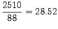
The time mean speed() is computed as:
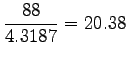
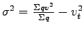
The space mean speed can be computed as:
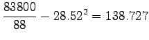
The standard deviation can be computed as:
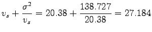
The time mean speed can also can also be computed as:
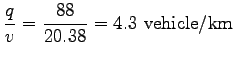
The density can be found as:
|
|
| | |
|
|
|