| |
| | |
|
In order to understand the concept of time mean speed and space mean speed,
following illustration will help.
Let there be a road stretch having two sets of vehicle as in
figure 1.
Figure 1:
Illustration of relation between time mean speed and space mean speed
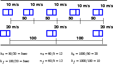 |
The first vehicle is traveling at 10m/s with 50 m spacing, and the second set
at 20m/s with 100 m spacing.
Therefore, the headway of the slow vehicle  will be 50 m divided by 10 m/s
which is 5 sec.
Therefore, the number of slow moving vehicles observed at A in one hour will be 50 m divided by 10 m/s
which is 5 sec.
Therefore, the number of slow moving vehicles observed at A in one hour  will be 60/5 = 12 vehicles.
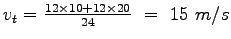
The density
will be 60/5 = 12 vehicles.
The density  is the number of vehicles in 1 km, and is the inverse of
spacing.
Therefore, is the number of vehicles in 1 km, and is the inverse of
spacing.
Therefore,
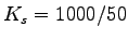 = 20 vehicles/km.
Therefore, by definition, time mean speed = 20 vehicles/km.
Therefore, by definition, time mean speed  is given by is given by
 .
Similarly, by definition, space mean speed is the mean of vehicle speeds over
time.
Therefore, .
Similarly, by definition, space mean speed is the mean of vehicle speeds over
time.
Therefore,
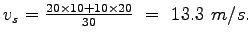 This is same as the harmonic mean of spot speeds obtained at location A; ie
 It may be noted that since harmonic mean is always lower than the arithmetic
mean, and also as observed, space mean speed is always lower than the time
mean speed.
In other words, space mean speed weights slower vehicles more heavily as they
occupy the road stretch for longer duration of time.
For this reason, in many fundamental traffic equations, space mean speed is
preferred over time mean speed.
It may be noted that since harmonic mean is always lower than the arithmetic
mean, and also as observed, space mean speed is always lower than the time
mean speed.
In other words, space mean speed weights slower vehicles more heavily as they
occupy the road stretch for longer duration of time.
For this reason, in many fundamental traffic equations, space mean speed is
preferred over time mean speed.
|
|
| | |
|
|
|