It is a famous relation showing θ as the unique function of ![]() . Eq. (4.5.10) is used to obtain the
. Eq. (4.5.10) is used to obtain the ![]() curve (Fig. 4.5.3) for
curve (Fig. 4.5.3) for ![]() .
.
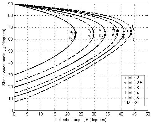
Fig. 4.5.3: ![]() curves for an oblique shock.
curves for an oblique shock.
The following inferences may be drawn from ![]() curves. It is seen that there is a maximum deflection angle
curves. It is seen that there is a maximum deflection angle ![]() .
.
- • For any given
 , if,
, if,  , the oblique shock will be attached to the body (Fig. 4.5.4-a). When
  , there will be no solution and the oblique shock will be curved and detached as shown in Fig. 4.5.4(b). The locus of
  can be obtained by joining the points (a1, b1, c1, d1, e1 and f1) in the Fig. 4.5.3.
• Again, if ![]() , there will be two values of
, there will be two values of ![]() predicted from
predicted from ![]() relation. Large value of
relation. Large value of ![]() corresponds to strong shock solution while small value refers to weak shock solution (Fig. 4.5.4-c). In the strong shock solution, M2 is subsonic while in the weak shock region, M2 is supersonic. The locus of such points (a2, b2, c2, d2, e2 and f2) as shown in Fig. 4.5.3, is a curve that also signifies the weak shock solution. The conditions behind the shock could be subsonic if θ becomes closer to
corresponds to strong shock solution while small value refers to weak shock solution (Fig. 4.5.4-c). In the strong shock solution, M2 is subsonic while in the weak shock region, M2 is supersonic. The locus of such points (a2, b2, c2, d2, e2 and f2) as shown in Fig. 4.5.3, is a curve that also signifies the weak shock solution. The conditions behind the shock could be subsonic if θ becomes closer to ![]() .
.
• If ![]() , it corresponds to a normal shock when
, it corresponds to a normal shock when ![]() and the oblique shock becomes a Mach wave when
and the oblique shock becomes a Mach wave when ![]() .
.
Fig. 4.5.4: (a) Attached shock; (b) Detached shock; (c) Strong and weak shock.