Next: Method of Undetermined Coefficients Up: Second Order and Higher Previous: Variation of Parameters Contents
This section is devoted to an introductory study of higher order linear
equations with constant coefficients. This is an extension of the study of
![]() order linear equations with constant coefficients
(see, Section 8.3).
order linear equations with constant coefficients
(see, Section 8.3).
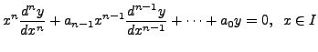
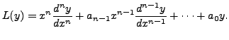
The standard form of a linear
![]() order differential equation
with constant coefficients is given by
order differential equation
with constant coefficients is given by
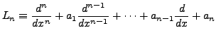
is a linear differential operator of order
 being real constants (called the coefficients of the
linear equation) and the function
being real constants (called the coefficients of the
linear equation) and the function
 is also a solution of (8.6.2).
Hence, if
is also a solution of (8.6.2).
Hence, if
is also a solution of (8.6.2). The solution
As in Section 8.3, we first take up the study of
(8.6.2). It is easy to note (as in Section 8.3)
that for a constant
![]()
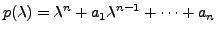
where,
Note that
![]() is of polynomial of degree
is of polynomial of degree ![]() with real coefficients.
Thus, it has
with real coefficients.
Thus, it has ![]() zeros (counting with multiplicities). Also, in case
of complex roots, they will occur in conjugate pairs. In view of this,
we have the following theorem. The proof of the theorem is omitted.
zeros (counting with multiplicities). Also, in case
of complex roots, they will occur in conjugate pairs. In view of this,
we have the following theorem. The proof of the theorem is omitted.
are the
are linearly independent solutions of (8.6.2), corresponding to the root
These are complex valued functions of
are also solutions of (8.6.2). Thus, in the case of
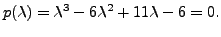
By inspection, the roots of
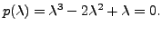
By inspection, the roots of
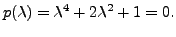
By inspection, the roots of
From the above discussion, it is clear that the linear homogeneous equation
(8.6.2), admits ![]() linearly independent solutions since the algebraic
equation
linearly independent solutions since the algebraic
equation
![]() has exactly
has exactly ![]() roots (counting with multiplicity).
roots (counting with multiplicity).
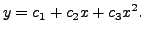
is called a general solution of (8.6.2), where
 and
and
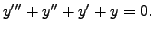
Then substituting
So,
We turn our attention toward the non-homogeneous equation (8.6.1).
If ![]() is any solution of (8.6.1) and if
is any solution of (8.6.1) and if  is the
general solution of the corresponding homogeneous equation (8.6.2),
then
is the
general solution of the corresponding homogeneous equation (8.6.2),
then

is a solution of (8.6.1). The solution
Solving an equation of the form (8.6.1) usually means to find a
general solution of (8.6.1). The solution ![]() is called a
PARTICULAR SOLUTION which may not involve any arbitrary constants.
Solving (8.6.1) essentially involves two steps (as we had seen
in detail in Section 8.3).
is called a
PARTICULAR SOLUTION which may not involve any arbitrary constants.
Solving (8.6.1) essentially involves two steps (as we had seen
in detail in Section 8.3).
Step 1: a) Calculation of the homogeneous solution ![]() and
and
b) Calculation of the particular solution ![]()
In the ensuing discussion, we describe the method of undetermined coefficients
to determine ![]() Note that a particular solution is not unique. In fact,
if
Note that a particular solution is not unique. In fact,
if ![]() is a solution of (8.6.1) and
is a solution of (8.6.1) and ![]() is any solution of
(8.6.2), then
is any solution of
(8.6.2), then ![]() is also a solution of (8.6.1).
The undetermined coefficients method is applicable for equations
(8.6.1).
is also a solution of (8.6.1).
The undetermined coefficients method is applicable for equations
(8.6.1).