Next: Higher Order Equations with Up: Second Order and Higher Previous: Non Homogeneous Equations Contents
In the previous section, calculation of particular integrals/solutions for some
special cases have been studied. Recall that the homogeneous part of the
equation had constant coefficients. In this section, we deal with a useful
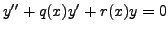
technique of finding a particular solution when the coefficients of the
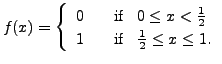
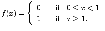
homogeneous part are continuous functions and the forcing function ![]() (or the non-homogeneous term) is piecewise continuous. Suppose
(or the non-homogeneous term) is piecewise continuous. Suppose ![]() and
and
![]() are two linearly independent solutions of
are two linearly independent solutions of
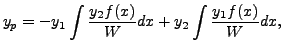
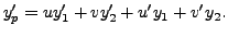
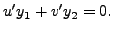
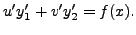
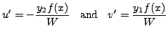
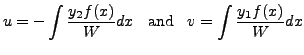
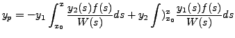
is a solution of (8.5.1) for any constants
As
Before, we move onto some examples, the following comments are useful.
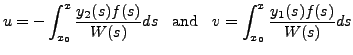
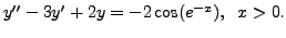
where
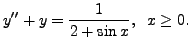
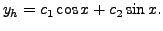
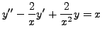
Here, the solutions
 are linearly independent over
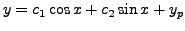
 by Theorem 8.5.1, is
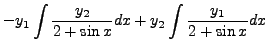
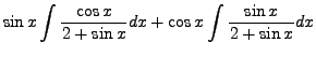
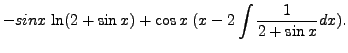
where
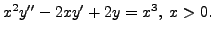
and two linearly independent solutions of the corresponding homogeneous part are
 and
and
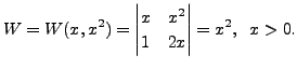
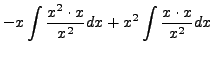
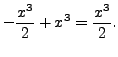
By Theorem 8.5.1, a particular solution
 |
|||
 |
 with
with