Non Homogeneous Equations

Throughout this section, $I$ denotes an interval in ${\mathbb{R}}.$ we assume that $q(\cdot), r(\cdot)$ and $f(\cdot)$ are real valued continuous function defined on $I.$ Now, we focus the attention to the study of non-homogeneous equation of the form

$$y^{\prime\prime} + q(x) y^\prime + r(x) y = f(x).$$ (8.4.1)

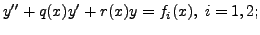
We assume that the functions $q(\cdot), r(\cdot)$ and $f(\cdot)$ are known/given. The non-zero function $f(\cdot)$ in (8.4.1) is also called the non-homogeneous term or the forcing function. The equation

$$y^{\prime\prime} + q(x) y^\prime + r(x) y = 0.$$ (8.4.2)

is called the homogeneous equation corresponding to (8.4.1).

Consider the set of all twice differentiable functions defined on $I.$ We define an operator $L$ on this set by

$$L(y) = y^{\prime\prime} + q(x) y^\prime + r(x) y.$$

Then (8.4.1) and (8.4.2) can be rewritten in the (compact) form

$$L(y) = f$$ (8.4.3)

$$L(y) = 0.$$ (8.4.4)

The ensuing result relates the solutions of (8.4.1) and (8.4.2).

THEOREM 8.4.1  

1. Let $y_1$ and $y_2$ be two solutions of (8.4.1) on $I.$ Then $y = y_1 - y_2$ is a solution of (8.4.2).
2. Let $z$ be any solution of (8.4.1) on $I$ and let $z_1$ be any solution of (8.4.2). Then $y = z+z_1$ is a solution of (8.4.1) on $I.$

Proof. Observe that $L$ is a linear transformation on the set of twice differentiable function on $I.$ We therefore have

$$L(y_1) = f \;\; {\mbox{ and }} \;\; L(y_2) = f.$$

The linearity of $L$ implies that $L(y_1 - y_2 ) = 0$ or equivalently, $y = y_1 - y_2$ is a solution of (8.4.2).

For the proof of second part, note that

$$L(z) = f \;\;{\mbox{ and }} \;\; L(z_1) = 0$$

implies that

$$L(z+z_1) = L(z) + L(z_1) = f.$$

Thus, $y = z+z_1$ is a solution of (8.4.1). height6pt width 6pt depth 0pt

The above result leads us to the following definition.

DEFINITION 8.4.2 (General Solution)   A general solution of (8.4.1) on $I$ is a solution of (8.4.1) of the form

$$y = y_h + y_p, \; x \in I$$

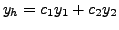
where $y_h = c_1 y_1 + c_2 y_2$ is a general solution of the corresponding homogeneous equation (8.4.2) and $y_p$ is any solution of (8.4.1) (preferably containing no arbitrary constants).

We now prove that the solution of (8.4.1) with initial conditions is unique.

THEOREM 8.4.3 (Uniqueness)   Suppose that $x_0 \in I.$ Let $y_1$ and $y_2$ be two solutions of the IVP

$$y^{\prime\prime} + q y^\prime + r y = f, \;\; y(x_0) = a, \;\; y^\prime(x_0) = b.$$ (8.4.5)

Then $y_1 = y_2$ for all $x \in I.$

Proof. Let $z = y_1 - y_2.$ Then $z$ satisfies

$$L(z) = 0, \;\; z(x_0) = 0, \;\; z^\prime(x_0) = 0.$$

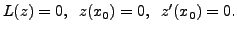
By the uniqueness theorem 8.1.9, we have $z \equiv 0$ on $I.$ Or in other words, $y_1 \equiv y_2$ on $I.$ height6pt width 6pt depth 0pt

Remark 8.4.4   The above results tell us that to solve (i.e., to find the general solution of (8.4.1)) or the IVP (8.4.5), we need to find the general solution of the homogeneous equation (8.4.2) and a particular solution $y_p$ of (8.4.1). To repeat, the two steps needed to solve (8.4.1), are:

1. compute the general solution of (8.4.2), and
2. compute a particular solution of (8.4.1).

   Then add the two solutions.

Step $1.$ has been dealt in the previous sections. The remainder of the section is devoted to step $2.,$ i.e., we elaborate some methods for computing a particular solution $y_p$ of (8.4.1).

EXERCISE 8.4.5  

1. Find the general solution of the following equations:
   1. $y^{\prime\prime} + 5 y^\prime = -5.$ (You may note here that $y = -x$ is a particular solution.)
   2. $y^{\prime\prime} - y = -2 \sin x.$ (First show that $y = \sin x$ is a particular solution.)
2. Solve the following IVPs:
   1. $y^{\prime\prime} + y = 2 e^x, \; y(0) = 0 = y^\prime(0).$ (It is given that $y = e^x$ is a particular solution.)
   2. $y^{\prime\prime} - y = -2 \cos x, \; \; y(0) = 0 , \; y^\prime(0)=1.$ (First guess a particular solution using the idea given in Exercise 8.4.5.1b )
3. Let $f_1(x)$ and $f_2(x)$ be two continuous functions. Let $y_i$ 's be particular solutions of
   $$y^{\prime\prime} + q(x) y^\prime + r(x) y = f_i(x), \; i=1,2;$$
   where $q(x)$ and $r(x)$ are continuous functions. Show that $y_1 + y_2$ is a particular solution of $y^{\prime\prime} + q(x) y^\prime + r(x) y = f_1(x) + f_2(x).$