Introduction

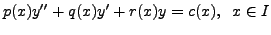
Second order and higher order equations occur frequently in science and engineering (like pendulum problem etc.) and hence has its own importance. It has its own flavour also. We devote this section for an elementary introduction.

DEFINITION 8.1.1 (Second Order Linear Differential Equation)   The equation

$$p(x) y^{\prime\prime} + q(x) y^\prime + r(x) y = c(x), \;\; x \in I$$ (8.1.1)

is called a SECOND ORDER LINEAR DIFFERENTIAL EQUATION.

Here $I$ is an interval contained in ${\mathbb{R}};$ and the functions $p(\cdot), q(\cdot), r(\cdot),$ and $c(\cdot)$ are real valued continuous functions defined on ${\mathbb{R}}.$ The functions $p(\cdot), q(\cdot),$ and $r(\cdot)$ are called the coefficients of Equation (8.1.1) and $c(x)$ is called the non-homogeneous term or the force function.

Equation (8.1.1) is called linear homogeneous if $c(x) \equiv 0$ and non-homogeneous if $c(x) \neq 0.$

Recall that a second order equation is called nonlinear if it is not linear.

EXAMPLE 8.1.2  

1. The equation
   $$y^{\prime\prime} + \sqrt{\frac{9}{\ell}} \sin y = 0$$
   is a second order equation which is nonlinear.
2. $y^{\prime\prime} - y = 0$ is an example of a linear second order equation.
3. $y^{\prime\prime} + y^\prime + y = \sin x$ is a non-homogeneous linear second order equation.
4. $a x^2 y^{\prime\prime} + b x y^\prime + c y = 0\; c \neq 0$ is a homogeneous second order linear equation. This equation is called EULER EQUATION OF ORDER 2. Here $a, b,$ and $c$ are real constants.

DEFINITION 8.1.3   A function $y$ defined on $I$ is called a solution of Equation (8.1.1) if $y$ is twice differentiable and satisfies Equation (8.1.1).

EXAMPLE 8.1.4  

1. $e^x$ and $e^{-x}$ are solutions of $y^{\prime\prime} - y = 0.$
2. $\sin x$ and $\cos x$ are solutions of $y^{\prime\prime} + y = 0.$

We now state an important theorem whose proof is simple and is omitted.

THEOREM 8.1.5 (Superposition Principle)   Let $y_1$ and $y_2$ be two given solutions of

$$p(x) y^{\prime\prime} + q(x) y^\prime + r(x) y = 0, \;\; x \in I.$$ (8.1.2)

Then for any two real number $c_1, c_2,$ the function $c_1 y_1 + c_2 y_2$ is also a solution of Equation (8.1.2).

It is to be noted here that Theorem 8.1.5 is not an existence theorem. That is, it does not assert the existence of a solution of Equation (8.1.2).

DEFINITION 8.1.6 (Solution Space)   The set of solutions of a differential equation is called the solution space.

For example, all the solutions of the Equation (8.1.2) form a solution space. Note that $y(x) \equiv 0$ is also a solution of Equation (8.1.2). Therefore, the solution set of a Equation (8.1.2) is non-empty. A moments reflection on Theorem 8.1.5 tells us that the solution space of Equation (8.1.2) forms a real vector space.

Remark 8.1.7   The above statements also hold for any homogeneous linear differential equation. That is, the solution space of a homogeneous linear differential equation is a real vector space.

The natural question is to inquire about its dimension. This question will be answered in a sequence of results stated below.

We first recall the definition of Linear Dependence and Independence.

DEFINITION 8.1.8 (Linear Dependence and Linear Independence)   Let $I$ be an interval in ${\mathbb{R}}$ and let $f, g : I \longrightarrow {\mathbb{R}}$ be continuous functions. we say that $f, g$ are said to be linearly dependent if there are real numbers $a$ and $b$ (not both zero) such that

$$a f(t) + b g(t) = 0 \;\; {\mbox{ for all }} \;\; t \in I.$$

The functions $f(\cdot), g(\cdot)$ are said to be linearly independent if $f(\cdot), g(\cdot)$ are not linear dependent.

To proceed further and to simplify matters, we assume that $p(x) \equiv 1$ in Equation (8.1.2) and that the function $q(x)$ and $r(x)$ are continuous on $I.$

In other words, we consider a homogeneous linear equation

$$y^{\prime\prime} + q(x) y^\prime + r(x) y = 0, \;\;\; x \in I,$$ (8.1.3)

where $q$ and $r$ are real valued continuous functions defined on $I.$

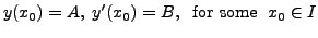
The next theorem, given without proof, deals with the existence and uniqueness of solutions of Equation (8.1.3) with initial conditions $y(x_0) = A, \; y^\prime(x_0) = B$ for some $x_0 \in I.$

THEOREM 8.1.9 (Picard's Theorem on Existence and Uniqueness)   Consider the Equation (8.1.3) along with the conditions

$$y(x_0) = A, \; y^\prime(x_0) = B, \; {\mbox{ for some }} \; x_0 \in I$$ (8.1.4)

where $A$ and $B$ are prescribed real constants. Then Equation (8.1.3), with initial conditions given by Equation (8.1.4) has a unique solution on $I.$

A word of Caution: NOTE THAT THE COEFFICIENT OF #MATH4130# MATHEND000# IN EQUATION () IS MATHEND000# BEFORE WE APPLY THEOREM , WE HAVE TO ENSURE THIS CONDITION.

An important application of Theorem 8.1.9 is that the equation (8.1.3) has exactly $2$ linearly independent solutions. In other words, the set of all solutions over ${\mathbb{R}},$ forms a real vector space of dimension $2.$

THEOREM 8.1.10   Let $q$ and $r$ be real valued continuous functions on $I.$ Then Equation (8.1.3) has exactly two linearly independent solutions. Moreover, if $y_1$ and $y_2$ are two linearly independent solutions of Equation (8.1.3), then the solution space is a linear combination of $y_1$ and $y_2$ .

Proof. Let $y_1$ and $y_2$ be two unique solutions of Equation (8.1.3) with initial conditions

$$y_1(x_0) = 1,\; y_1^{\prime}(x_0) = 0, \;\;{\mbox{ and }} \;\; y_2(x_0) = 0, \; y_2^{\prime}(x_0) = 1 \; {\mbox{ for some }}\; x_0 \in I.$$ (8.1.5)

The unique solutions $y_1$ and $y_2$ exist by virtue of Theorem 8.1.9. We now claim that $y_1$ and $y_2$ are linearly independent. Consider the system of linear equations

$$\alpha y_1(x) + \beta y_2(x) = 0,$$ (8.1.6)

where $\alpha$ and $\beta$ are unknowns. If we can show that the only solution for the system (8.1.6) is $\alpha=\beta = 0$ , then the two solutions $y_1$ and $y_2$ will be linearly independent.

Use initial condition on $y_1$ and $y_2$ to show that the only solution is indeed $\alpha=\beta = 0$ . Hence the result follows.

We now show that any solution of Equation (8.1.3) is a linear combination of $y_1$ and $y_2$ . Let $\zeta$ be any solution of Equation (8.1.3) and let $d_1 = \zeta(x_0)$ and $d_2 = \zeta^\prime(x_0).$ Consider the function $\phi$ defined by

$$\phi(x) = d_1 y_1(x) + d_2 y_2(x).$$

By Definition 8.1.3, $\phi$ is a solution of Equation (8.1.3). Also note that $\phi(x_0) = d_1$ and $\phi^\prime(x_0) = d_2.$ So, $\phi$ and $\zeta$ are two solution of Equation (8.1.3) with the same initial conditions. Hence by Picard's Theorem on Existence and Uniqueness (see Theorem 8.1.9), $\phi(x) \equiv \zeta(x)$ or

$$\zeta(x) = d_1 y_1(x) + d_2 y_2(x).$$

Thus, the equation (8.1.3) has two linearly independent solutions. height6pt width 6pt depth 0pt

Remark 8.1.11  

1. Observe that the solution space of Equation (8.1.3) forms a real vector space of dimension $2.$
2. The solutions $y_1$ and $y_2$ corresponding to the initial conditions
   $$y_1(x_0) = 1,\; y_1^{\prime}(x_0) = 0, \;\;{\mbox{ and }} \;\; y_2(x_0) = 0, \; y_2^{\prime}(x_0) = 1 \; {\mbox{ for some }}\; x_0 \in I,$$
   are called a FUNDAMENTAL SYSTEM of solutions for Equation (8.1.3).
3. Note that the fundamental system for Equation (8.1.3) is not unique.
   Consider a $2 \times 2$ non-singular matrix $A = \begin{bmatrix}a & b \\ c & d \end{bmatrix}$ with $a, b, c, d \in {\mathbb{R}}.$ Let $\{y_1, y_2\}$ be a fundamental system for the differential Equation 8.1.3 and ${\mathbf y}^t = [y_1, \; y_2 ].$ Then the rows of the matrix 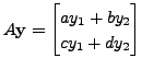$A {\mathbf y}= \begin{bmatrix}a y_1 + b y_2 \\ c y_1 + d y_2 \end{bmatrix}$ also form a fundamental system for Equation 8.1.3. That is, if $\{y_1, y_2\}$ is a fundamental system for Equation 8.1.3 then $\{ a y_1 + b y_2, c y_1 + d y_2 \}$ is also a fundamental system whenever $ad - bc = \det (A) \neq 0.$

EXAMPLE 8.1.12   $\{1, {\mathbf x}\}$ is a fundamental system for $y^{\prime\prime} = 0.$
Note that $\{1 - {\mathbf x}, 1+ {\mathbf x}\}$ is also a fundamental system. Here the matrix is $\begin{bmatrix}1 & -1 \\ 1 & 1 \end{bmatrix}.$

EXERCISE 8.1.13  

1. State whether the following equations are SECOND-ORDER LINEAR or SECOND-ORDER NON-LINEAR equaitons.
   1. $y^{\prime\prime} + y \sin x = 5.$
   2. $y^{\prime\prime} + (y^\prime)^2 + y \sin x = 0.$
   3. $y^{\prime\prime} + y y^\prime = -2.$
   4. $(x^2 + 1) y^{\prime\prime} + (x^2 + 1)^2 y^\prime - 5 y = \sin x.$
2. By showing that $y_1 = e^x$ and $y_2 = e^{-x}$ are solutions of
   $$y^{\prime\prime} - y = 0$$
   conclude that $\sinh x$ and $\cosh x$ are also solutions of $y^{\prime\prime} - y = 0.$ Do $\sinh x$ and $\cosh x$ form a fundamental set of solutions?
3. Given that $\{ \sin x, \cos x\}$ forms a basis for the solution space of $y^{\prime\prime} + y = 0,$ find another basis.