Next: Orthogonal Projections and Applications Up: Inner Product Spaces Previous: Definition and Basic Properties Contents
Let ![]() be a finite dimensional inner product space.
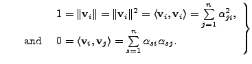
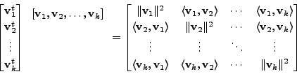
Suppose
be a finite dimensional inner product space.
Suppose
![]() is a linearly independent subset of
is a linearly independent subset of ![]() Then the Gram-Schmidt orthogonalisation
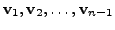
process uses the vectors
Then the Gram-Schmidt orthogonalisation
process uses the vectors
![]() to construct new
vectors
to construct new
vectors
 such that
![]() for
for ![]()
![]() and
and
![]() for
for
![]() This process
proceeds with the following idea.
This process
proceeds with the following idea.
Suppose we are given two vectors
![]() and
and
![]() in a plane. If we
want to get vectors
in a plane. If we
want to get vectors
![]() and
and
![]() such that
such that
![]() is a unit
vector in the direction of
is a unit
vector in the direction of
![]() and
and
![]() is a unit vector
perpendicular to
is a unit vector
perpendicular to
 then they can be obtained in the following
way:
then they can be obtained in the following
way:
Take the first vector
![]() Let
Let ![]() be the angle between the
vectors
be the angle between the
vectors
![]() and
and
![]() Then
Then
 Defined
 Then
Then
 is a vector perpendicular
to the unit vector
is a vector perpendicular
to the unit vector
![]() , as we have removed the component of
, as we have removed the component of
![]() from
from
![]() .
So, the vectors that we are interested in are
.
So, the vectors that we are interested in are
![]() and
and
![]()
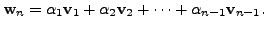
This idea is used to give the Gram-Schmidt Orthogonalisation process which we now describe.
 are
already obtained, we compute
are
already obtained, we compute
For ![]() we have
we have
![]() Since
Since
![]() and
and
Hence, the result holds for
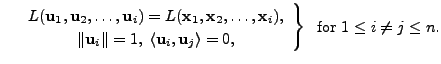
Let the result hold for all
![]() That is, suppose we are given any set of
That is, suppose we are given any set of
![]() linearly independent vectors
linearly independent vectors
![]() of
of ![]() Then by the inductive assumption,
there exists a set
Then by the inductive assumption,
there exists a set
![]() of vectors satisfying the following:
of vectors satisfying the following:
Now, let us assume that we are given a set of ![]() linearly independent vectors
linearly independent vectors
![]() of
of ![]() Then by the inductive assumption,
we already have vectors
Then by the inductive assumption,
we already have vectors
 satisfying
On the contrary, assume that
![]() Then
there exist scalars
Then
there exist scalars
![]() such that
such that
So, by (5.2.2)
Thus, by the third induction assumption,
This gives a contradiction to the given assumption that the set of vectors
So,
![]() . Define
. Define
![]() .
Then
.
Then
![]() . Also, it can be easily verified that
. Also, it can be easily verified that
![]() for
for
![]() .
Hence, by the principle of mathematical induction, the proof of the theorem is complete.
height6pt width 6pt depth 0pt
.
Hence, by the principle of mathematical induction, the proof of the theorem is complete.
height6pt width 6pt depth 0pt
We illustrate the Gram-Schmidt process by the following example.
 Let
Let
Hence,
 Let
Let
 |
 |
||
We claim that in this case,

Since, we have chosen the smallest ![]() satisfying
satisfying
for
As
So, by definition of

Therefore, in this case, we can continue with the Gram-Schmidt process
by replacing
 by
by

Let
is an
Also, observe that the conditions
![]() and
and
![]() for
for
![]() implies that
implies that
 |
|||
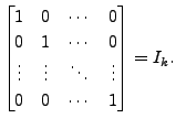 |
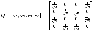
Perhaps the readers must have noticed that the inverse of ![]() is its transpose. Such matrices are called
orthogonal matrices and they have a special role to play.
is its transpose. Such matrices are called
orthogonal matrices and they have a special role to play.
It is worthwhile to solve the following exercises.
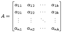
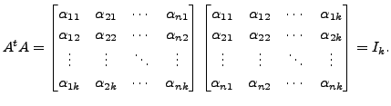
![$\displaystyle A = [{\mathbf u}_1, {\mathbf u}_2, \ldots, {\mathbf u}_n] = \begi...
...s & \vdots & \ddots & \vdots \\ a_{n1} & a_{n2} & \cdots & a_{nn}
\end{bmatrix}$](img2454.png)
where
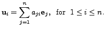
Prove that
 Hence deduce that
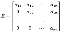
In case, ![]() is non-singular, the diagonal entries of
is non-singular, the diagonal entries of ![]() can
be chosen to be positive. Also, in this case, the decomposition is
unique.
can
be chosen to be positive. Also, in this case, the decomposition is
unique.
Let the columns of ![]() be
be
 The Gram-Schmidt
orthogonalisation process applied to the vectors
The Gram-Schmidt
orthogonalisation process applied to the vectors
 gives the vectors
![]() satisfying
satisfying
By using (5.2.5), we get
![$\displaystyle [{\mathbf u}_1, {\mathbf u}_2, \ldots, {\mathbf u}_n] \begin{bmat...
...dots & \vdots &
\ddots & \vdots \\ 0 & 0 & \cdots & {\alpha}_{nn} \end{bmatrix}$](img2468.png) |
|||
![$\displaystyle \biggl[ {\alpha}_{11} {\mathbf u}_1, \; {\alpha}_{12} {\mathbf u}...
...pha}_{22}{\mathbf u}_2, \ldots,
\sum_{i=1}^n {\alpha}_{in}{\mathbf u}_i \biggr]$](img2469.png) |
|||
The proof doesn't guarantee that for
![]()
![]() is positive. But this can be achieved by replacing the vector
is positive. But this can be achieved by replacing the vector
![]() by
by
 whenever
 is negative.
Uniqueness: suppose
![]() then
then
![]() Observe the following properties of
upper triangular matrices.
Observe the following properties of
upper triangular matrices.
Suppose we have matrix
![]() of dimension
of dimension
![]() with
with
![]() Then by Remark
5.2.3.2, the application of the Gram-Schmidt
orthogonalisation process yields a set
Then by Remark
5.2.3.2, the application of the Gram-Schmidt
orthogonalisation process yields a set
![]() of orthonormal vectors of
of orthonormal vectors of
![]() In this case, for each
In this case, for each
![]() we have
we have
Hence, proceeding on the lines of the above theorem, we have the following result.
 That is, the columns
of
That is, the columns
of
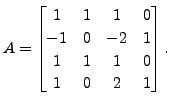
 Find an orthogonal
matrix
Find an orthogonal
matrix
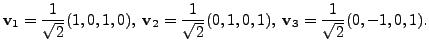
We now compute
 If
we denote
If
we denote
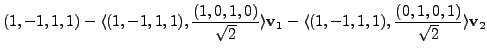
 then by the Gram-Schmidt process,
and
The readers are advised to check that
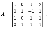
 Find a
 matrix
  and an upper triangular matrix
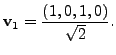
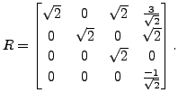
Let
![]() Define
Define
![]() Let
Let
![]() Then
Then
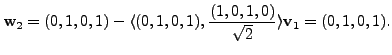
Hence,
 Let
Let
So, we again take
So,
 Hence,
![$\displaystyle Q = [{\mathbf v}_1, {\mathbf v}_2, {\mathbf v}_3] = \begin{bmatri...
...{bmatrix}2 & 1 & 3 & 0
\\ 0 & 1 & -1 & 0 \\ 0 & 0 & 0 & \sqrt{2} \end{bmatrix}.$](img2515.png)
The readers are advised to check the following:
 upper triangular matrix with
 Find the corresponding
functions,
Find the corresponding
functions, ![$ A = \biggl[ [{\mathbf x}]_{{\cal B}}, \; [{\mathbf x}_2]_{{\cal B}}, \; \ldots, \; [{\mathbf x}_n]_{{\cal B}}
\biggr].$](img2542.png) Then prove that
Then prove that A K Lal 2007-09-12
![\includegraphics[scale=1]{gramschmidt.eps}](img2367.png)