Density Distribution of Atomic Orbitals.

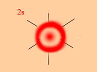
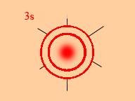
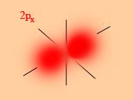
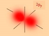
An accurate way of visualizing the orbitals is through a plot of the charge densities, which are given by e | | ² or the probability densities, | | ² . The plots of | | ² in 3 dimensions are shown in fig 5.3. The regions where | | ² is large are shown by dense dots and the regions where the density is small are shown by orbitals thin or sparse dots. The densities for 1s, 2s, 3s, 2p_x , 2p_y , 2p_z , 3d _{x y} , 3d_x² _{- y}² , 3d_{y z} , 3d_{z x} and 3d_z ² are shown in figs 5.3 (a) to 5.3 (k). The spherical nodes of 2s and 3s can be easily identified. The planar nodes of 2p and four of the 3d orbitals can easily be identified. For the 3d _z ² orbital, the nodes are conical in shape and the angles of the two conical surfaces from the vertical z- axis are given by the two roots of the function (1/2) ( 3 cos ² – 1 ). Another useful way of visualizing the orbitals is through boundary surfaces.

c)

d)