where is the maximum angular velocity of the rotor to be achieved and is the time taken for the same. On integration the above equation gives

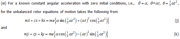
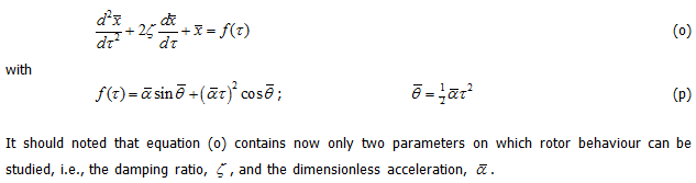
It should be noted that above equations are now uncoupled and linear and can be solved independent of each other. The forcing is general in nature, hence, to get the response either of equations can be time integrated by using numerical integrations, e.g., the Newmark's method.

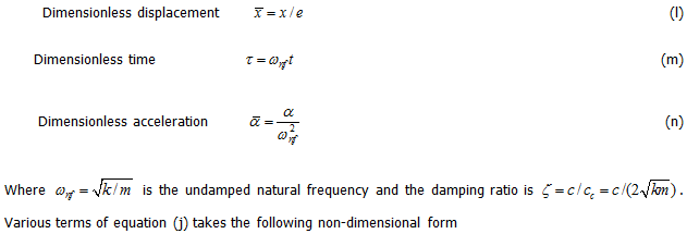
By introducing the following non-dimensional parameters

          

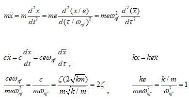
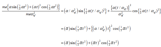
So that equation of motion in non-dimensional form (j) takes finally the following form

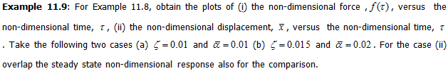
Solution : Equation (o) of example 11.9 is time integrated by the Newmark method (Appendix 11A). Various plots are shown in Figs. 11.36 to 11.37 for two different operating angular accelerations given in the problem. Fig 11.36(a) and (b) are transient displacement and velocity variation with respect to the time. Fig.11.36(c) and (d) are phase plots (i.e., the velocity versus the displacement), respectively, while approaching towards the resonance (the amplitude is continuously increasing) and terminating away from the resonance (the amplitude has decreasing trend). Fig. 11.36(e) represents the steady state displacement with time for a particular frequency, and Fig. 11.36(f) represents the steady state displacement with frequency. Fig. 11.36(g) represents the steady state and transient displacements with frequency, which are overlapped in a single plot. For the clarity of the plot only the amplitude of the steady state response is plotted with respect to the frequency of excitation. However, in the transient case since the response is continuously changing, hence, the actual response with actual angular speed corresponding to the time of the response is shown (which is exactly the same in the shape as that of Fig. 11.37(a) with the change of only the abscissa axis from time to the angular speed). It can be observed that in transient the maximum amplitude occurs well away from the resonance condition that of the steady state case, however, with a lesser amplitude. The main aim of giving such angular acceleration is very clear from this plot that if resonance is passed with a certain angular acceleration, the time to build up high amplitude at resonance could be avoided. Figs. 11.37 have similar trends as that of the previous case.