Solving Eq. (6.3.16) and Eq. (6.3.17) one may write Eq. (6.3.15) as 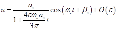..........................................................................(6.3.18)

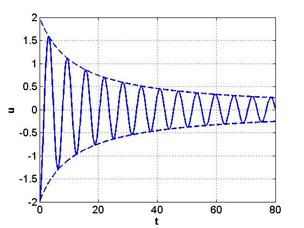
Figure 6.3.2 : Time response of the system with quadratic damping.

Using Eq. (6.3.18) the time response is shown in Fig. 6.3.2. It may be noted that unlike the linear system the response does not decreases exponentially but decreases algebraically. The corresponding Matlab code is given in Matlab code 6.3.3.

Matlab code 6.3.3:

% plotting of quadratic damping. (Eq. 6.3.18)
clc
clear all
a0=2;
ep=.1;
t=0:0.1:80;
omega=1;
beta=-3.15;
a=a0./(1+(4*ep*omega*a0*t)/(3*pi));
u=a.*cos(omega*t+beta);
plot(t,u,t,a, '--' ,t,-a, '--' )
% title('SYSTEM WITH QUADRATIC DAMPING')
set(findobj(gca, 'Type' , 'line' ), 'Color' , 'b' , 'LineWidth' ,2);
set(gca, 'FontSize' ,14)
xlabel( 't' , 'fontsize' ,14, 'fontweight' , 'b' );
ylabel( 'u' , 'fontsize' ,14, 'fontweight' , 'b' );
grid on

System with Coulomb damping

In this case the equation of motion of the system can be given by

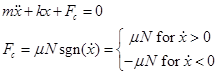...............................................................................(6.3.19)