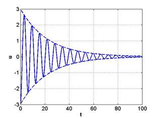
Figure 6.3.1(b): Time response of the system with linear damping.

Using Eq. (6.3.10) the time response is shown in Fig. 6.3.1(b ). It may be noted that the response decreases exponentially. The corresponding Matlab code is given below

Matlab code 6.3.1:

%Free Vibration response of a linear single degree of freedom system

x0=0.1;
xt0=0.001;
wn=2;
zeta=1.5;
t=0:0.001:20;

%overdamped

z1=-zeta+sqrt(zeta^2-1);
z2=-zeta-sqrt(zeta^2-1);
z3=2*wn*sqrt(zeta^2-1);
A=(xt0-z2*wn*x0)/z3;
B=(-xt0+z1*wn*x0)/z3;
x1=A*exp(z1*wn*t)+B*exp(z2*wn*t);

%critically damped

x2=(x0+(xt0+wn*x0)*t).*exp(-wn*t)

%underdamped

zt=0.2 %Damping factor
wd=wn*sqrt(1-zt^2);
x3=exp(-zt*wn*t).*(((xt0+zt*wn*x0)/wd).*sin(wd*t)+x0*cos(wd*t));

plot(t,x1,'r',t,x2,'b',t,x3,'g','linewidth',2)
grid on

set(gca,'FontSize',15) % For changing fontsize of tick no
xlabel('\bf Time','Fontsize',15)
ylabel('\bf x','Fontsize',15)