This equation is same as the expression one may obtain by finding the complementary function of the differential equation (6.3.2). Using the and as the initial displacement and velocity respectively, one may write Eq. (6.3.10) as

............................................. (6.3.11)

Where the damped natural frequency

For over damped ( ) system one may use the following expressions for the response.

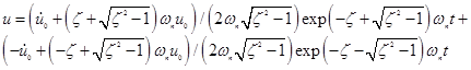..........................(6.3.12)

For critically damped ( ) system one may write the response as follows.

.................................................................................(6.3.13)

A Matlab code is given below to plot for response of a system under damped, critically damped and over damped conditions as shown in figure 6.3.1.

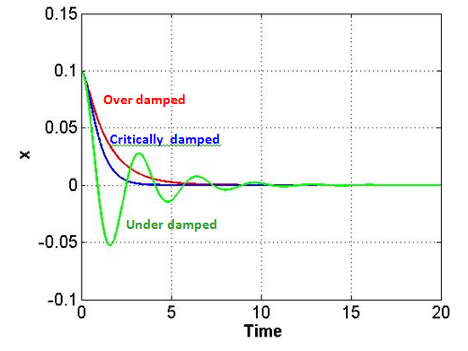
Figure 6.3.1(a): Time response of a linear single degree of freedom with viscous damping.