The pressure and temperature of the fluid upstream and down stream of the restriction are measured with suitable manometers and thermometers [Fig. 1.20].

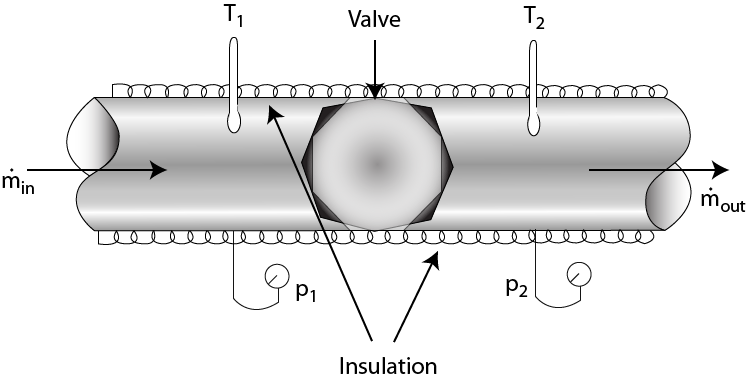
Fig. 1.20 Joule Thompson effect

Let p_i and T_i be the arbitrarily chosen pressure and temperature before throttling and let us assume that they are constant. By operating the restriction (say, a valve) the fluid is throttled successively to different pressures and temperatures p_ƒ1, T_ƒ1; p_ƒ2, T_ƒ2; p_ƒ3, T_ƒ3 and so on. These are then plotted on the T -p plane [Fig. 1.3].

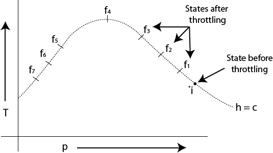
Fig. 1.21 Isenthalpic states of a gas

All the points on this curve represent equilibrium states of some constant mass of the fluid. The curve passing through all these points is an isenthalpic curve or isenthalpe.

The initial pressure and temperature of the fluid (p_i, T_i) are then set to new values and the fluid is throttled by controlling the restriction. Thus by throttling to different states we can have a family of isenthalpes for the fluid [Fig. 1.22]. The curve passing through the maxima of these isenthalpes is called the inversion curve.

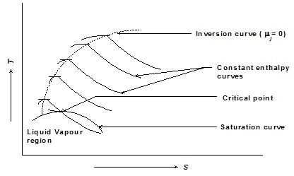
Fig. 1.22 Inversion and saturation curves on T-s plot

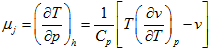
The numerical value of the slope of an is enthalpe on the T - p diagram at any point is called the Joule –Thompson coefficient µ_j.

1.190

Locus of all points at which µ_j is zero is the inversion curve. The region inside the inversion curve where µ_j is negative is called the heating region and where µ_j is positive is called the cooling region.

The difference in enthalpy between two neighboring equilibrium states is

dh = Tds + vdp

1.191

and the second T - dS relation (per unit mass)

1.192

1.193

The second term in the above equation stands only for a real gas, because for an ideal gas dh = C_pdT

1.194