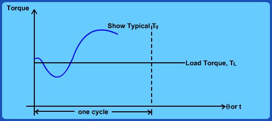
Fig 5.6 Supply and load torque Representative

Let us look at Fig. 5.6 which is a general representation of load and supply torques over a cycle and investigate the dynamics of the system. From point A to B in the cycle, the load torque exceeds the available torque. So the shaft speed falls from A to B. During B-C, the load torque will further slow down the shaft making point C perhaps the minimum speed point. During C-D, the system gains in speed as the supply torque is much more than the load torque. During D-E, the system again slows down gradually coming back to the speed at A (beginning of cycle). Thus we could identify the points in the cycle that correspond to the maximum and minimum speed and write the following energy balance equation:

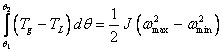                                       (5.6)

where correspond to the points of maximum and minimum speeds and J is the mass moment of inertia of the system including crank shaft, other rotating parts along with flywheel. Assuming that the speed fluctuation is actually quite small after the installation of a flywheel, we could approximately write:

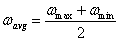                                                                          (5.7)

If we define a coefficient of fluctuation of speed k_s as:

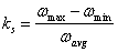                                                                            (5.8)

We can re-write eq. (5.6) as:

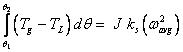                                                   (5.9)

In order to simplify our calculations, we could further assume that the mass moment of inertia of the flywheel ( ) is perhaps much larger than that of the other rotating parts and hence simply take .