The straight line asymptotes of the Bode plot can be drawn using the following.

• Up to ω_w= 0.997 rad/sec, the magnitude plot is a straight line with slope - 20 dB/decade.At ω_w= 0.01 rad/sec,the magnitude is $20 \log_{10}(10.02) - 20 \log_{10}(0.01) = 60$ dB.

• From ω_w= 0.997 rad/sec to ω_w= 20 rad/sec, the magnitude plot is a straight line with slope - 20 - 20 = - 40 dB/decade.

• Since both of the zeros will contribute same to the magnitude plot, after ω_w= 20 rad/sec, the slope of the straight line will be - 40 + 20 + 20 = 0 dB/decade.

The asymptotic magnitude plot is shown in Figure 1.

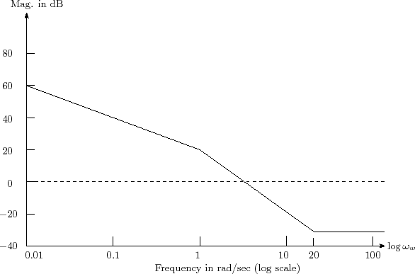$\begin{figure} \begin{center} \input{m5l5fig1.pstex_t} \end{center} \end{figure}$

Figure 1: Bode asymptotic magnitude plot for Example 1

One should remember that the actual plot will be slightly different from the asymptotic plot. In the actual plot, errors due to straight line assumptions is compensated.

Phase plot is drawn by varying the frequency from 0.01 to 100 rad/sec at regular intervals. The phase angle contributed by one zero will be canceled by the other. Thus the phase will vary from

- 90° (270°) to - 180° (180°).