Pole zero map of the uncompensated system is shown in Figure 3. Sum of angle contributions at the desired pole is $A =\theta_1-\theta_2-\theta_3$ , where $\theta_1$ is the angle by the zero, , and $\theta_2$ and $\theta_3$ are the angles contributed by the two poles, 0.82 and 1 respectively.

From the pole zero map as shown in Figure 3, the angles can be calculated as $\theta_1=16.5^{o}$ , $\theta_2=124.9^{o}$ and $\theta_3=138.1^{o}$ .

Net angle contribution is $A=16.5^{o}-124.9^o-138.1^{o}-109.8^{0}=-247.5^{0}$ . But from angle criterion a point will lie on root locus if the total angle contribution at that point is $\pm 180^o$ . Angle deficiency is $-247.5^{o}+180^{o}=67.5^{o}$

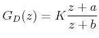
Controller pulse transfer function must provide an angle of 66.5°. Thus we need a Lead Compensator. Let us consider the following compensator.

$\displaystyle G_{D}(z)=K\frac{z+a}{z+b}$

If we place controller zero at z = 0.82 to cancel the pole there, we can avoid some of the calculations involved in the design. Then the controller pole should provide an angle of $124.9^{o}-67.5^{o}=57.4^{o}$ .

Once we know the required angle contribution of the controller pole, we can easily calculate the pole location as follows.

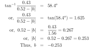
The pole location is already assumed at . Since the required angle is greater than $\tan^{-1}(0.43/0.52)=39.6^o$ we can easily say that the pole must lie on the right half of the unit circle. Thus b should be negative. To satisfy angle criterion,

The controller is then written as 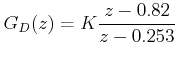$G_D(z)=K\dfrac{z-0.82}{z-0.244}$ . The root locus of the compensated system (with controller) is shown in Figure 4.

$\includegraphics[width=12cm]{m5l2rl2.eps}$

Figure 4: Root locus of the compensated system