Question and Answers
Question:
The lower bound estimate algorithm discussed in Section 4.3 may not always give a sharp bound. Suggest suitable modifications and show that better bounds can be obtained. Also show using an example, how benefit is achieved in branch and bound algorithm using the modification .
Answer:
The following 4 steps were present in the lower bound estimate algorithm discussed in Section 4.3. The modification is highlighted as bold.
1. Add a field w to each row, whose value is equal to the number of 1's in the row
2. Choose the row with minimum w . Let it be  . If there are multiple rows with same value, choose the one from the top.
3. Delete all rows  such that and have at least one column where both of them have a 1. Also, delete . If, after deletion no more rows remain, then check if there exists a column PI say, such that PI has all 1s. If there is no such column then 1 needs to be added the lower bound.
4. Repeat step 2 and 3 until no more rows remain.
The motivation of the extension is explained by the following matrix.
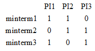
In the above matrix, if we apply the lower bound estimate algorithm discussed in Section 4.2, then we get the answer as 1; the algorithm stops after 1 iteration because row1 is selected and row2 and row3 get eliminated. However, it may be noted one column cannot cover the three rows because no column PI exists, such that PI has all 1s. Therefore, in this case, we increment the cost by 1; two rows can cover. It may be noted that if the matrix has more rows and columns, then the addition required in the cost may be more than 2. However to keep the algorithm simple we compromise on accuracy and add just 1; calculating more accurate value to be added, requires more computation steps.
Now we illustrate the benefit of using the modified lower bound computation algorithm in the Branch and Bound technique.
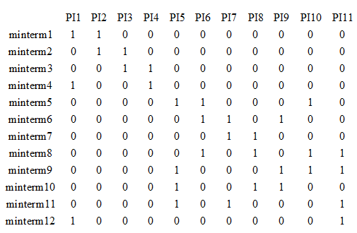
Let us again consider the constraint matrix given in example of Subsection 4.4 (given below). If we apply the modified lower bound estimate algorithm, we get Lower Bound = 4 comprising {1, 3,5,7} (same as the original algorithm of Section 4.3).