The way of computing the lower bound depends on the particular problem. We shall discuss a lower bound algorithm that applies to the covering problem. It is obvious that a careful choice of the lower bound criterion is important. Ideally, the criterion should provide an accurate estimate of the real minimum cost incurred in completing the current solution. At the same time, the computation of the bound should be fast. So, most of the lower bound estimation algorithms are fast heuristics, that may not provide a sharp bound. So the branch and bound algorithm for unate covering problem generally provides near optimal solutions. However, due to the lower bound estimation heuristics the execution time is low.

Before we turn our attention to the computation of the lower bound for the unate covering problem, we now look at the steps for the branch-and-bound algorithm for the unate covering problem.

1.  Execute the lower bound computation algorithm on the constraint matrix. The “Initial Lower Bound” is the Lower Bound. Current Cost is set to 0.

2.  Select or de-select a column PI (i.e., a path in the solution space corresponding PI=1 or PI=0). If a column PI is selected then add PI to the cover and add cost 1 to the Current Cost. Apply reduction techniques (essential columns, row and column dominance) to the constraint matrix. For all essential columns, add them to the cover and increase Current Cost by the number of essential columns. If the problem is now reduced to a terminal case (because of selection of a column), then check whether the solution thus found is better than (or at least at par) the “Initial Lower Bound” (i.e., Initial Lower Bound Current cost). If so, the cover is returned and algorithm is terminated.

3.  On the reduced matrix, again compute the lower bound. Add the lower bound value to the Current Cost. If there is still a chance of getting an optimal solution, identify a column to be selected/de-selected from the reduced matrix and go to Step-2; execute step-2 by selecting/de-selecting the column being marked.

If the value of lower bound + Current Cost is higher than Initial Lower Bound, then there is no point in exploring that path. Undo selection or de-selection of the column done last (in Step-2), consequent selection/de-selection of columns (due to matrix reduction) and addition in Current cost. Go to step-2 and traverse another path by selecting or de-selecting an alternative column.

4.3  Computation of the Lower Bound

As discussed in the last sub-section, the branch and bound algorithm needs a procedure that can provide a quick estimate of the minimum number of columns required for a cover. This lower bound helps the algorithm to retract (to other branches by selecting appropriate column) if the estimated solution cost is higher than the expected one, without actually exploring the full path.

We now address the problem of computing a lower bound approximation to the cost of covering a constraint matrix in terms of number of columns. Before the discussion, some definitions and a theorem are introduced.

Definition 11: In a given covering matrix C , suppose that two rows have no nonzero columns in common, we say these two rows are independent (that is, column-disjoint).

It is obvious that we need two different columns to cover these two rows. Generalizing this argument, if a matrix has n rows that are disjoint (pair wise), we need at least n columns to cover the whole matrix. In this case, the rows are said to form an independent set of rows. In the constraint matrix given below, rows corresponding to minterm1, minterm3 and minterm5 are independent as they do not have a common column that has 1. Similarly, rows corresponding to minterm2, minterm4 and minterm6 are independent. So, we need at least three columns to cover the matrix. The lower bound in this case is 3.

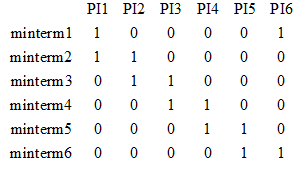
For cyclic matrices, lower bound is 2 or more, as shown in the following theorem.