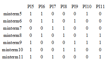
In this matrix Lower Bound = 2 comprising {5,7}. So if we explore on this matrix the solution cost lower bound is 2+2=4. As this value is equal to that of the Lower Bound on the initial matrix, we explore on the search space. Let us now consider column PI5. With PI5 being taken, the following happens in the matrix
• rows minterm9, minterm10, and minterm11 are covered,
• columns PI9 (by PI6), PI10 (PI6) and PI11 (by PI6) are dominated
The left edge from root note indicates PI5 being taken (Figure 2). Also in the edge it is marked that “PI9', PI0',PI1'”—this indicates that because of taking PI5, PI9, PI10 and PI11 get eliminated.
After reduction (i.e., taking PI5 and eliminating PI92, PI10, PI1) we get the following matrix. As of now the cost of the solution is 3 (PI1, PI3,PI5).
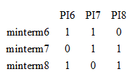
In this matrix Lower Bound = 1 comprising {6}. So if we explore on this matrix the solution cost lower bound is 3+1=4. As this value is equal to that of the Lower Bound on the initial matrix, we explore on the search space. If we consider PI6, the following happens in the matrix
• row minterm8 is covered,
• Column PI7 or PI8 needs to be taken in the cover.
This is the terminal case as all rows are covered. This is solution is {PI1,PI3,PI5,PI6,PI7} (left edge of PI7) in Figure 2 or {PI1,PI3,PI5,PI6,PI8} (right edge of PI7). In both the solutions, the cost is 5, which is higher than the initial expected lower bound. Therefore, we need to retract. We may select an alternative path where, PI6=0 (right edge of PI6). It is easy to observe that in this case the solution is {PI1,PI3,PI5,PI7,PI8}; as the cost is 5 we retract. We may select an alternative path where, PI5=0 (right edge of PI5).
Similarly, the whole tree (as in Figure 2) can be created. In this example, if the whole tree is created, it may be noted that the cost at all branches (solution space) is 5. Therefore, the whole tree will be explored and in the end, it will be concluded that the lower bound (=4) given by the estimate is not sharp and a solution (of cost 5) will be taken as cover. However, it is not always the case. In the Question and Answer part of the lecture we will provide a modified lower bound estimate algorithm and show how, in the same example (being considered in this sub-section) some paths need not be explored
5. Conclusions
In this lecture, we discussed, given an arbitrary SOP formula, how to obtain a minimal cost Boolean function representation of the same. Cost in this case is the number of literals being taken in the product terms of the equation. The minimal cost representation can be used directly for logic gate level implementation, followed by Backend flow of VLSI design process. In this lecture, all discussions were regarding single output functions; for multiple output functions slight modifications are required, for which the reader is referred to [7]. However, there is an important issue about the techniques discussed in this lecture. It may be noted that at many phases of the schemes, we need to enumerate all minterms; if an SOP involves n variables then the number of minterms may be 2n. This limits the practical usage of the techniques discussed in this lecture. In the >> lecture, we will discuss a heuristic scheme for obtaining a minimal cost Boolean function representation of an SOP. The heuristic is much faster than the techniques discussed here, however, the cost of the solution may be higher.