Destination choice models

The postulate of travel behaviour on which this model is based is that destination $j$ will be chosen from origin $i$ for a particular trip purpose if the perceived utility derived from choosing $j$ is greater than the perceived utility derived from choosing any other destination. It is further assumed that, $u_i(j)$, the utility derived from destination $j$ by an individual (or a group of similar individuals) in origin $i$ has two components: (i) the deterministic component, $v_i(j)$ and (ii) the stochastic component $e_i(j)$. The deterministic component is the approximate utility that can be obtained from the destination, given the destination's in situ attributes and the impedances. On the other hand, the stochastic component can be thought of as an approximation of the random variability assumed to be present in the utility because of the fact that this is a quantity which is perceived by humans. Mathematically,

$$u_i(j) = v_i(j) + e_i(j)$$ (16)

Since, $u_i(j)$ is a stochastic quantity, the answer to the question as to which destination provides a greater utility will be probabilistic. Keeping this in mind the basic postulate described in the earlier paragraph is modified thus: the probability that destination $j$ will be chosen from origin $i$ for a particular trip purpose is equal to the probability that the perceived utility derived from $j$ is greater than the perceived utility derived from each of the other destinations. Mathematically,

$$\pi_{ij} = {\rm Prob.}(u_i(j) > u_i(k) , \forall k \neq j)$$ (17)

That is,

$$\begin{eqnarray*} \pi_{ij} & = & {\rm Prob.}\{v_i(j) + e_i(j) > v_i(k) + e_i(k),... ...m Prob.}\{e_i(k) < v_i(j) - v_i(k) + e_i(j), \forall k \neq j \} \end{eqnarray*}$$

Once $\pi_{ij}$ are obtained, the trip distribution between any $i$ and $j$ can be obtained by multiplying $T_i$ with $\pi_{ij}$.

It is, however, clear from the above equations that the exact nature of $\pi_{ij}$ will depend on the assumptions about the nature of the $e_i(k)$'s. If it is assumed that (i) $e_i(k)$'s are distributed identically for each $k$, (ii) that they are independent, and (iii) that they are distributed according to the Gumbel distribution, i.e.

$${\rm Prob.} \{e_i(k) < z\} = e^{-\theta e^{-z}}$$

then the resulting expression for $\pi_{ij}$ can be obtained as follows:

$$\pi_{ij} = \int_{-\infty}^{\infty}\prod_{\forall k \neq j}e^... ...) + x)}} \left\{ \theta e^{-x}e^{-\theta e^{-x}} \right \} dx$$ (18)

now realizing that when $k=j$ then $e^{-\theta e^{v_i(j) - v_i(k) + x}} = e^{-\theta e^{-x}}$ one can rewrite Equation  as

$$\pi_{ij} = \int_{-\infty}^{\infty}e^{-\theta e^{-x} \sum_k e^{-(v_i(j) - v_i(k))}} \theta e^{-x} dx$$ (19)

now substituting $g= - \theta e^{-x}$ and $w=\sum_k e^{-(v_i(j) - v_i(k))}$, one obtains

$$\pi_{ij} = \frac{1}{w}$$ (20)

or

$$\pi_{ij} = \frac{e^{v_i(j)}}{\sum_k e^{v_i(k)}}$$ (21)

The form for $\pi_{ij}$ given in Equation  is known as the multinomial logit model.

Example

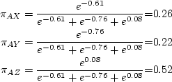
For the data given in the previous example problem and assuming

$$v_A(j) = 0.5 \times \mbox{{\rm Shopping area of Zone} $j$\ {\... ... m.}} - 0.23 \times \mbox{{\rm Distance to} $j$\ {\rm in km.}}$$

determine the trip distribution using the multinomial logit model.

Solution

For the given data, $v_A(X) = -0.61$, $v_A(Y) = -0.76$, and $v_A(Z) = 0.08$. Hence, the probabilities are:

$$\begin{eqnarray*} \pi_{AX} = \frac{e^{-0.61}}{e^{-0.61}+e^{-0.76}+e^{0.08}} & = ... ...{AZ} = \frac{e^{0.08}}{e^{-0.61}+e^{-0.76}+e^{0.08}} & = & 0.52 \end{eqnarray*}$$

and the trip distribution is given by:

$$\begin{eqnarray*} t_{AX} = 0.26 \times 1200 & = & 312\\ t_{AY} = 0.22 \times 1200 & = & 264 \\ t_{AZ} = 0.52 \times 1200 & = & 624 \end{eqnarray*}$$

Discussion: Instead of assuming a Gumbel distribution for the random terms, if it is assumed that they are distributed normally then the resulting form for $\pi_{ij}$ is called the Probit model. This model is, however, a lot more cumbersome than the Logit model. For a detailed and extensive discussion on the Probit model one may refer to Kanafani [#!kan1!#].

Another point which may be mentioned here is about the calibration of destination choice models. The parameters which need to be calibrated are the parameters of the function $v_i(j)$. Since the choice models give the probability of choosing a destination from a given origin, one may use the maximum likelihood estimation technique to estimate the parameters. Note that the likelihood function will the same as that given in Equation .