The postulate of travel behaviour on which this model is based, from Stouffer [221], is that the probability of choice of a particular destination (from a given origin for a particular trip purpose) is proportional to the opportunities for trip-purpose satisfaction at the destination and inversely proportional to all such opportunities that are closer to the origin. The inverse proportionality to closer opportunities can be interpreted as proportionality to the probability that none of the closer destinations (opportunities) are chosen. Thus, in this model, the in-situ attractive properties of the destination are modeled as opportunities and the impedances are measured in terms of the number of opportunities which are closer.
In order to formulate the postulate as a mathematical model, the following notation are used:
L: Constant of proportionality (or calibration constant).
J : Total number of destinations.
j: Index indicating the position of a destination (from the given origin), j =1 for the nearest destination and j = J for the farthest.
 :Cumulative function of opportunities up to and including the :Cumulative function of opportunities up to and including the  destination
from origin i. destination
from origin i.
 : Probability that a destination is chosen from the ith origin by the time the jth
destination is reached. : Probability that a destination is chosen from the ith origin by the time the jth
destination is reached.
πij: Probability that the jth destination is chosen from the ith origin.
Based on the postulate, the following expression can be written:
 |
(11) |
This relation states that a small addition in opportunities  after the jth destination causes a correspondingly small increase in the probability after the jth destination causes a correspondingly small increase in the probability  . This increase is proportional to the probability that no destination is chosen by the jth destination and the amount of additional opportunities. . This increase is proportional to the probability that no destination is chosen by the jth destination and the amount of additional opportunities.
Using  (since it is assumed that (since it is assumed that  ) and solving the differential equation we get ) and solving the differential equation we get
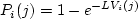 |
(12) |
and since, by definition,
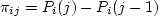 , we have , we have |
|
 |
(13) |
Note, however, nothing guarantees that  . In fact, . In fact,
 could be interpreted as the probability that no destination is chosen. This, however, poses a problem in the sequential demand analysis framework because if no destination is chosen then it leads to a situation where a trip is produced but does not go anywhere. In order to correct this anomaly, the πij obtained in Equation 12 is modified by adding a constraint which states that a destination must be chosen from the set of available destinations thereby precluding the possibility of not choosing any destination. Mathematically this can be done in one of two ways, both leading to the same result. We could use the Bayes theorem and determine the probability that destination j is chosen given that a destination is chosen or we could simply normalize the πij's obtained in Equation 13 by dividing the individual πij's with could be interpreted as the probability that no destination is chosen. This, however, poses a problem in the sequential demand analysis framework because if no destination is chosen then it leads to a situation where a trip is produced but does not go anywhere. In order to correct this anomaly, the πij obtained in Equation 12 is modified by adding a constraint which states that a destination must be chosen from the set of available destinations thereby precluding the possibility of not choosing any destination. Mathematically this can be done in one of two ways, both leading to the same result. We could use the Bayes theorem and determine the probability that destination j is chosen given that a destination is chosen or we could simply normalize the πij's obtained in Equation 13 by dividing the individual πij's with
 . In either case the modified πij, written as . In either case the modified πij, written as  , is given by, , is given by,
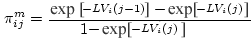 |
(14) |
Note that the denominator can be looked upon as either (i) the probability a destination is chosen, P(J)or (ii)
. (The reader should verify these claims).
Once the  are obtained the trips between i and j can be obtained as: are obtained the trips between i and j can be obtained as:
 |
(15) |
Example
For the 1200 shopping trips from Zone A, three destinations exist. The destinations are Zones X, Y, and Z. The shopping areas available in each of the zones and their distances from Zone A are given in Table 2. Assuming a proportionality constant of 0.35 and assuming a thousand square meter of shopping area as one opportunity determine the trip distribution from Zone A.
Table 2 : Data for the example 2 on intervening opportunities model
Zone |
Shopping area |
Distance from Zone A |
|
(in '000 sq.m.) |
(in km) |
X |
2.0 |
7.0 |
Y |
4.0 |
12.0 |
Z |
2.0 |
4.0 |
Solution
First, the destinations should be arranged from the closest to the farthest; in this case, j = 1 for Zone Z, j = 2 for Zone X, and j = 3 for Zone Y. Since there are only 3 destinations, j = 3.
Next, Vi (j) need to be determined;  , and , and  and and  . .
Using Equation 14 the ,  , ,  and and  are calculated as follows: are calculated as follows:
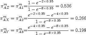
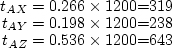
Therefore, the trip distribution from Zone A is given by
Discussion: Since the model gives the probability of choosing a destination from a given origin we may employ the maximum likelihood technique to calibrate the constant L. The likelihood function is similar to that given in Equation 10. However, it is seen that assumption of a constant L is not very good for most problems. A varying L adds complexity to the model and its calibration. For a more detailed discussion on intervening opportunity models one may see Kanafani [132] or Stouffer [221] or Ruiter [197].
|