The trip-distribution models strive to predict the number of trips that will be made between a pair of zones for a particular trip-purpose. These models try to mathematically describe the destination-choice phase of the sequential demand analysis procedure. There are various models of trip distribution. However, most of them incorporate the same basic factors which affect the number of trips between an origin zone and a destination zone. The models differ in their characterization of these factors and in the way these factors are assumed to affect the trip distribution.
The factors (for any given trip-purpose) which affect the number of trips between two zones are:
- The number of trips produced by the origin zone.
- The degree to which the in-situ attributes of the destination zone attract trip makers. The attributes which gain importance vary with the trip purpose. For example, if one is modeling the number of shopping trips attracted to a zone then the type of attributes of the zone which assume importance will be the total shopping floor area, number of retail outlets, and the like. On the other hand, if one is modeling the number of work trips attracted to a zone then the type of attributes of the zone which assume importance will be the number of offices, the type of offices, and so forth.
- The factors that inhibit travel between a pair of zones. These factors could be, travel time, travel distance, travel cost, and so on.
Four different models are presented here. These are (i) Gravity model, (ii) Intervening opportunities model, (iii) Choice model, and (iv) Entropy Model.
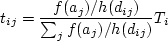
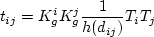
The Gravity model uses the following basic form to determine the trips between an origin zone i and a destination zone j. That is,
t ij =  |
(3) |
where,
Ti is the total number of trips being produced by origin zone i
aj is a set of in-situ attributes of the destination zone j which attract trip makers
dij is a set of factors which inhibit travel between two zones
 is a calibration constant is a calibration constant
 and and  are positive monotonically increasing functions. are positive monotonically increasing functions.
Note that
 is basically the trip attractions of Zone j. is basically the trip attractions of Zone j.
The expression
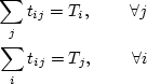
may be thought of as a factor which distributes the total trips produced by a zone among all the possible destination zones. In this sense, the sum of the expression over all destinations should be equal to unity. Thus,
 |
(4) |
The above equation implies that,
 |
(5) |
Substituting, the expression for in Equation 3, the following relation, often referred to as the origin constrained gravity model, is obtained:
 |
(6) |
Sometimes, in the gravity model, the number of trips attracted to a zone (when such data is independently available),  , is used as a surrogate for , is used as a surrogate for . When such a substitution is done the gravity model is typically written as . When such a substitution is done the gravity model is typically written as
 |
(7) |
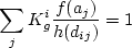
Very often, in this case the following two constraints are imposed on the gravity model to obtain the two calibration constants.
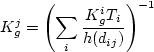
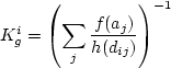
 On imposition of the two constraints, the constants
  and and  are obtained as: are obtained as:
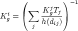 |
(8) |
Example
Consider the following six-zone model of a town. Zones 1, 2, and 3 are fully residential areas and Zones 4, 5 and 6 are purely shopping areas. The shopping areas, shopping trips attracted (per day), the shopping trips produced (per day) and the travel distances are as shown in Table 1. The cells which have a ``-'' imply that those data are irrelevant to the problem. Determine the trip distribution between the zones for the following different scenarios:
(a) Use the origin-constrained gravity model, assuming to be a linear function of the shopping area (in square meters) with a slope of 0.01 and constant term of 10. Also assume  to be dij2 where dij is the distance in km. to be dij2 where dij is the distance in km.
(b) Use the origin-destination constrained gravity model with same relevant assumptions same as those in (a).
Table 1 : Data for the example on Gravity Model
Zone |
Shop
Area (  ) |
Trips
Produced |
Trips
Attracted |
Distance (km) to |
1 |
2 |
3 |
4 |
5 |
6 |
1 |
- |
1000 |
- |
- |
- |
- |
4 |
2 |
7 |
2 |
- |
1000 |
- |
- |
- |
- |
3 |
1 |
6 |
3 |
- |
2000 |
- |
- |
- |
- |
5 |
2 |
6 |
4 |
1000 |
- |
800 |
4 |
3 |
5 |
- |
- |
- |
5 |
2000 |
- |
2000 |
2 |
1 |
2 |
- |
- |
- |
6 |
3000 |
- |
1200 |
7 |
6 |
6 |
- |
- |
- |
Solution
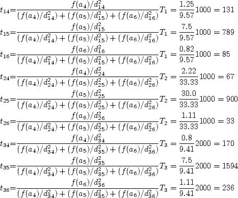
(a)
The trips of interest here are  , where , where  and and
 . Also note, as per the problem description f(aj) = 0.01 x (shopping area in m2) + 10, and . Also note, as per the problem description f(aj) = 0.01 x (shopping area in m2) + 10, and
 . The trips are given by Equation 6. . The trips are given by Equation 6.
(b)
In this case, the only difference from (a) is that the trips are given by Equation 7 and the constants of Equation 7 are given by Equations 8 and 9. The initial value of Kig is assumed to be the square root of the corresponding values obtained in (a). These values of Kig are used in Equation 9 to obtain a set of Kig values which are in turn used in Equation 8 to obtain a new set of Kig values. The process continues till all the  and values converge. The final values of and obtained are as follows: and values converge. The final values of and obtained are as follows:
Final values of
 , and , and  and and 
Final values of
 , ,  and and 
Using these values of and in Equation 7, the following tij values are obtained:
 , and , and  and and 
 , and , and  and and 
 , and , and  and and 
The reader must verify that for the above trips
 and and 
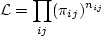
Discussion: It may be pointed out here that the expression 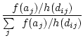 in Equation 6 may be viewed as
  , the probability that destination j is chosen from origin i. Once such a view is taken, then the Maximum likelihood technique can be used to estimate the parameters of the gravity model. If observations on the trip distribution between different origin-destination pairs are made and denoted as , the probability that destination j is chosen from origin i. Once such a view is taken, then the Maximum likelihood technique can be used to estimate the parameters of the gravity model. If observations on the trip distribution between different origin-destination pairs are made and denoted as  , then the likelihood function can be written as , then the likelihood function can be written as
 |
(10) |
Other constraints like
could be accounted for by adding the constraint to the likelihood function and constructing a Lagrangian.
|