Mixed boundary condition
We can also specify a mixed boundary condition in the form given below.
|
(12.25) |
This is also known as Type III boundary condition and is the linear combination of Type I and Type II boundary condition.
Initial condition
For time dependent problem, an initial condition for the head field h(x,y,z,t = 0) has to be specified. This is known as initial condition.
Fig. 12.3 shows the flow domain between two observation wells in case of a confined aquifer. The lines CF and DE represent equpotential lines of potential φ0 and φL respectively. Therefore on these two boundaries, Dirchlet boundary is to be applied. On the other hand at top and bottom of the surfaces of the aquifer are impervious. The lines CD and EF represent the no flow boundary. As such the Neumann boundary condition is to be applied on these two sides. Fig. 12.4 shows the aquifer with boundary conditions.
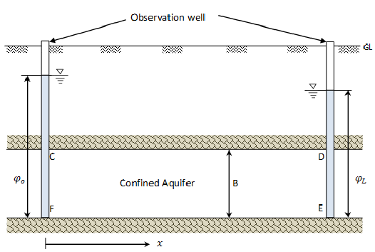 |
Fig. 12.3 Flow domain between observation wells |
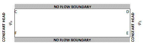 |
Fig. 12.4 Confined aquifer with boundary condition |