When the contaminant is reactive with the soil, the velocity of its travel may be less than the seepage velocity due to the retention process. To take this into account, relative ionic velocity (v_s/v_ion) is represented as

v_ion is the average velocity of reactive (non-conservative) contaminant species. For a non-reactive (conservative) contaminant, K_d will be negligible and hence v_sis equal to v_ion. Eq. 3.19 is valid only for saturated soil where porosity is equal to volumetric water content (θ). For unsaturated soil n is replaced by θ.

Determination of hydrodynamic dispersion and retardation coefficient

             A simple soil column test set up can be used to determine hydrodynamic dispersion and retardation coefficient simultaneously in the laboratory. A detailed description of these test procedures are discussed in the literature (Rowe et al. 1988). The soil sample is packed in the soil column with the compaction state expected in the field. The soil sample is saturated with water and the required contaminant solution of particular concentration is transferred on top of the compacted soil. Depending upon the test facilities, the flow of contaminant solution can be under constant head or under constant flow rate. 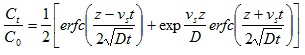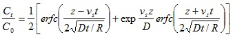Constant flow rate is possible only for high permeable soil. The contaminant solution after flowing through the soil is collected as effluent from the bottom of the column. The effluent is collected at regular intervals of time, filtered and analyzed for concentration. This measured concentration is designated as C_t (concentration at time t. Concentration variation of effluent can be related to time or pore volume. Once the test is over, the soil is sliced and the concentration sorbed on soil mass is determined. This will give the concentration variation with depth. Therefore, measured C_t can be obtained as a function of time, pore volume or depth. The solution to the governing differential equation (Eq. 3.19) can be best fitted to the experimental data to obtain the values of R and D. Analytical solution for Eq. 3.19 for simple boundary conditions given below is represented by Eqs. 3.20 and 3.21 for non-reactive and reactive contaminants, respectively. The solution is applicable for barrier which is assumed to be infinitely deep and subject to a constant source concentration.
Initial condition C (z, 0) = 0   z >0

Boundary conditions C (0, t) = C_o (initial concentration)   t ≥ 0
                                 C (∞, t) = 0 t ≥0

3.20

3.21

             For a given liner, it is essential to check whether the provided thickness is sufficient or not. For this purpose, the parameters governing contaminant transport such as v_s, D and R is obtained as discussed above for the liner material and model contaminant used. v_s is obtained by determining discharge velocity and knowing the compaction state. Numerical or analytical modelling is performed to determine the fate of model contaminant (position of contaminant with respect to space and time). For 1-D modelling as discussed above, space refers to depth. Based on the numerical modelling, it is checked whether the liner of given thickness and properties will be able to contain the contaminant for the given design life. It is expected that the concentration of contaminant reaching groundwater aquifer should not exceed the safe drinking water standards for the specified design or operational life. In case, it exceeds then the thickness or the material need to be reconsidered till it becomes safe. In certain cases, groundwater table is assumed at the bottom of the liner as worst case scenario. This means that the role of natural soil below liner is not considered. In the above modelling, the deterioration of liner material with aging is not considered. The modelling is done with a gross assumption that the material properties remain same with age.