Ei = vieψ |
2.2 |
where vi is the ionic valence, e is the electronic charge (=1.602 x 10⁻¹⁹ C) and ψ is the electrical potential at a point. ψ is defined as the work done to bring a positive unit charge from a reference state to the specified point in the electric field. Potential at the surface is denoted as ψ0. ψ is mostly negative for soils because of the negative surface charge. As distance from charged surface increases, ψ decreases from ψ0 to a negligible value close to reference state. Since ψ = 0 close to reference state, Ei0 = 0.
Therefore, Ei0 - Ei = -vieψ and Eq. 2.1 can be re-written as
ni = |
2.3 |
Eq. 2.3 relates ion concentration to potential as shown in Fig. 2.9.
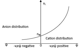 |
| Fig. 2.9 Ion concentration in a potential field (modified from Mitchell and Soga 2005) |
In Fig. 2.9 anion distribution is marked negative due to the reason that vi and ψ are negative and hence -vieψ will be negative. For cations, vi is positive and ψ is negative and hence -vieψ will be positive. For negatively charged clay surface, ni,cations > ni0 and ni,anions < ni0.
One dimensional Poisson equation (Eq. 2.4) relates electrical potential ψ, charge density ρ in C/m3 and distance (x). ε is the static permittivity of the medium (C2J-1m-1 or Fm-1).
|
2.4 |

ρ = eΣvini = e(v+n+-v-n-) |
2.5 |
ni is expressed as ions per unit volume, + and – subscript indicates cation and anion. Substituting Eq. 2.3 in 2.5
ρ = eΣvi |
2.6 |
Hence,
|
2.7 |
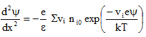
Eq. 2.7 represents differential equation for the electrical double layer adjacent to a planar surface. This equation is valid for constant surface charge. Solution of this differential equation is useful for computation of electrical potential and ion concentration as a function of distance from the surface.
Different models representing double layer (Yong 2001)
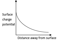
A) Helmholtz double layer: This model follows the simplest approximation that surface charge of clays are neutralized by opposite sign counter ions placed at a distance of “d” away from the surface. The surface charge potential decreases with distance away from the surface as shown in Fig. 2.10.
|
|
| Fig. 2.10 Variation of surface charge potential with distance from clay surface (modified from Mitchell and Soga 2005) |